The HLOOKUP function in Microsoft Excel is a powerful horizontal lookup tool that searches for values in the top row of a table and returns corresponding data from rows below. Unlike its vertical counterpart VLOOKUP, HLOOKUP works with horizontally organized data structures, making it essential for financial models, quarterly reports, and data arranged in row format.
What is HLOOKUP Function?
HLOOKUP stands for “Horizontal Lookup” and is designed to search for a specific value in the first row of a data range, then return a value from a specified row in the same column. This function proves invaluable when working with data organized horizontally rather than vertically.
HLOOKUP Syntax
The HLOOKUP function follows this syntax structure:
=HLOOKUP(lookup_value, table_array, row_index_num, [range_lookup])Parameters Explained:
- lookup_value: The value you want to search for in the first row of the table
- table_array: The range containing your data table
- row_index_num: The row number from which to return a value (1 for first row, 2 for second row, etc.)
- range_lookup: Optional parameter – TRUE for approximate match, FALSE for exact match
Step-by-Step HLOOKUP Tutorial
Basic HLOOKUP Example
Consider a sales data table organized horizontally:
| Product | Laptop | Phone | Tablet | Watch |
| Price | $999 | $699 | $399 | $299 |
| Stock | 25 | 50 | 30 | 75 |
To find the price of a “Phone”, use this formula:
=HLOOKUP("Phone", A1:E3, 2, FALSE)This returns $699 because “Phone” is found in row 1, and we’re requesting the value from row 2 (Price row).
Advanced HLOOKUP Techniques
Using Cell References
Instead of hardcoding values, reference cells for dynamic lookups:
=HLOOKUP(G1, A1:E3, 3, FALSE)Where G1 contains the product name you want to lookup, and row 3 returns stock information.
Approximate Match with Sorted Data
When using TRUE for range_lookup, ensure your first row is sorted in ascending order:
=HLOOKUP(750, A1:F2, 2, TRUE)This finds the largest value less than or equal to 750 in the first row.
HLOOKUP vs VLOOKUP: Key Differences
| Feature | HLOOKUP | VLOOKUP |
|---|---|---|
| Search Direction | Horizontal (across rows) | Vertical (down columns) |
| Lookup Row/Column | First row | First column |
| Return Parameter | Row index number | Column index number |
| Data Organization | Data in rows | Data in columns |
Common HLOOKUP Errors and Solutions
#N/A Error
This error occurs when the lookup value isn’t found. Solutions include:
- Verify the lookup value exists in the first row
- Check for extra spaces or formatting differences
- Use IFERROR to handle missing values gracefully
=IFERROR(HLOOKUP("Product", A1:E3, 2, FALSE), "Not Found")#REF! Error
Occurs when row_index_num exceeds the table range. Ensure your row index doesn’t exceed the table height.
#VALUE! Error
Results from incorrect data types or invalid parameters. Double-check your syntax and parameter types.
Practical HLOOKUP Applications
Financial Modeling
HLOOKUP excels in financial models where data is organized by time periods:
=HLOOKUP("Q2 2024", A1:F5, 3, FALSE)This retrieves specific quarterly data from horizontally arranged financial statements.
Performance Dashboards
Create dynamic dashboards that pull metrics based on selected criteria:
=HLOOKUP($B$1, Dashboard!$A$1:$M$10, ROW(A4), FALSE)Inventory Management
Track product information across multiple attributes organized horizontally:
=HLOOKUP(ProductCode, Inventory!A1:Z5, 4, FALSE)HLOOKUP Best Practices
Data Organization Tips
- Keep lookup values in the first row without duplicates
- Maintain consistent data formatting across rows
- Sort data ascending when using approximate match
- Avoid blank cells in the lookup row
Performance Optimization
- Use exact match (FALSE) whenever possible for accuracy
- Limit table array size to necessary data only
- Consider using structured table references for clarity
- Replace with INDEX-MATCH for better flexibility
Alternative Functions to HLOOKUP
INDEX and MATCH Combination
More flexible than HLOOKUP, allowing left-to-right lookups:
=INDEX(2:2, MATCH("Phone", 1:1, 0))XLOOKUP Function
Available in Excel 365, XLOOKUP provides enhanced lookup capabilities:
=XLOOKUP("Phone", 1:1, 2:2)Troubleshooting HLOOKUP Issues
Data Type Mismatches
Ensure lookup values match the data type in your table. Text formatted as numbers won’t match actual numbers.
Hidden Characters
Use TRIM and CLEAN functions to remove hidden spaces and characters:
=HLOOKUP(TRIM(CLEAN(A1)), B1:F5, 2, FALSE)Case Sensitivity
HLOOKUP is not case-sensitive by default, but formatting differences can cause issues. Standardize text case using UPPER or LOWER functions.
Advanced HLOOKUP Formulas
Multiple Criteria Lookup
Combine HLOOKUP with other functions for complex lookups:
=HLOOKUP(A1&B1, CHOOSE({1;2}, C1:F1&C2:F2, C3:F3), 2, FALSE)Dynamic Row Index
Use MATCH to create dynamic row references:
=HLOOKUP("Product", A1:F10, MATCH("Price", A:A, 0), FALSE)Conclusion
The HLOOKUP function remains a cornerstone tool for horizontal data analysis in Excel. While newer functions like XLOOKUP offer enhanced capabilities, understanding HLOOKUP ensures compatibility across Excel versions and provides a solid foundation for data lookup operations. Master these techniques to efficiently extract insights from horizontally organized datasets and build more dynamic, responsive spreadsheet models.
Practice with different data structures and scenarios to build confidence in applying HLOOKUP effectively. Remember to always validate your results and consider error handling to create robust, professional spreadsheet solutions.


