The LOOKUP function in Microsoft Excel is a powerful search tool that allows you to find specific values within your data sets quickly and efficiently. Whether you’re working with large databases, financial records, or simple lists, understanding how to use LOOKUP functions can dramatically improve your productivity and data analysis capabilities.
What is the Excel LOOKUP Function?
The LOOKUP function searches for a value in a single row or column and returns a corresponding value from the same position in another row or column. It’s designed to work with sorted data and provides a fundamental way to retrieve information based on search criteria.
Excel actually offers three main types of LOOKUP functions:
- LOOKUP – The basic lookup function
- VLOOKUP – Vertical lookup for searching columns
- HLOOKUP – Horizontal lookup for searching rows
Basic LOOKUP Function Syntax
The basic LOOKUP function has two forms: vector form and array form.
Vector Form Syntax
=LOOKUP(lookup_value, lookup_vector, result_vector)Parameters:
- lookup_value: The value you want to search for
- lookup_vector: A single row or column range to search in
- result_vector: A single row or column range containing return values
Array Form Syntax
=LOOKUP(lookup_value, array)Parameters:
- lookup_value: The value you want to search for
- array: A range containing both lookup and return values
How LOOKUP Function Works
The LOOKUP function operates by scanning through the lookup range to find the largest value that is less than or equal to your lookup value. This is why your data must be sorted in ascending order for the function to work correctly.
When LOOKUP finds a match (or the closest smaller value), it returns the corresponding value from the same position in the result range.
Step-by-Step LOOKUP Examples
Example 1: Basic Price Lookup
Let’s say you have a product list with quantities and corresponding prices:
| Quantity | Price per Unit |
|---|---|
| 1 | $10.00 |
| 10 | $9.50 |
| 50 | $9.00 |
| 100 | $8.50 |
To find the price for 75 units, you would use:
=LOOKUP(75, A2:A5, B2:B5)This returns $9.00 because 75 falls between 50 and 100, and LOOKUP returns the value associated with 50 (the largest value less than or equal to 75).
Example 2: Grade Lookup System
For a grading system where you want to assign letter grades based on numerical scores:
| Minimum Score | Grade |
|---|---|
| 0 | F |
| 60 | D |
| 70 | C |
| 80 | B |
| 90 | A |
For a score of 85, use:
=LOOKUP(85, A2:A6, B2:B6)This returns “B” because 85 falls between 80 and 90.
VLOOKUP: Vertical Data Search
VLOOKUP is the most commonly used lookup function, perfect for searching data organized in columns.
VLOOKUP Syntax
=VLOOKUP(lookup_value, table_array, col_index_num, [range_lookup])Parameters:
- lookup_value: Value to search for
- table_array: Range containing the data
- col_index_num: Column number to return data from
- range_lookup: TRUE for approximate match, FALSE for exact match
VLOOKUP Example
Employee database lookup:
| Employee ID | Name | Department | Salary |
|---|---|---|---|
| 101 | John Smith | Sales | $45,000 |
| 102 | Jane Doe | Marketing | $52,000 |
| 103 | Mike Johnson | IT | $58,000 |
To find the department for employee 102:
=VLOOKUP(102, A2:D4, 3, FALSE)This returns “Marketing” (column 3 in the range).
HLOOKUP: Horizontal Data Search
HLOOKUP works similarly to VLOOKUP but searches horizontally across rows instead of vertically down columns.
HLOOKUP Syntax
=HLOOKUP(lookup_value, table_array, row_index_num, [range_lookup])HLOOKUP Example
Monthly sales data arranged horizontally:
| Month | Jan | Feb | Mar | Apr |
|---|---|---|---|---|
| Sales | $25,000 | $28,000 | $22,000 | $31,000 |
| Expenses | $15,000 | $16,000 | $14,000 | $18,000 |
To find March expenses:
=HLOOKUP("Mar", B1:E3, 3, FALSE)This returns $14,000 (row 3 in the range).
Common LOOKUP Function Errors and Solutions
#N/A Error
Cause: Lookup value not found or data not sorted properly.
Solution: Check data sorting and verify lookup value exists.
#REF! Error
Cause: Column or row index number exceeds the range.
Solution: Verify your index numbers are within the table range.
#VALUE! Error
Cause: Data type mismatch or incorrect syntax.
Solution: Ensure lookup value matches data types in the lookup range.
Advanced LOOKUP Techniques
Two-Way Lookup
Combine INDEX and MATCH functions for more flexible lookups:
=INDEX(data_range, MATCH(row_lookup, row_range, 0), MATCH(col_lookup, col_range, 0))Approximate Match vs. Exact Match
Understanding when to use TRUE (approximate) vs. FALSE (exact) in the range_lookup parameter:
- TRUE/1: Finds closest match, requires sorted data
- FALSE/0: Finds exact match, works with unsorted data
Wildcard Lookups
Use wildcards with VLOOKUP for partial matches:
=VLOOKUP("John*", A:B, 2, FALSE)This finds any name starting with “John”.
Best Practices for LOOKUP Functions
Data Organization
- Keep lookup columns on the left for VLOOKUP
- Sort data appropriately for approximate matches
- Remove duplicate values in lookup columns
- Use consistent data formatting
Performance Optimization
- Use exact match (FALSE) when possible for better performance
- Limit table array size to necessary data only
- Consider using INDEX/MATCH for complex lookups
- Avoid volatile functions in lookup formulas
Error Handling
Use IFERROR to handle potential lookup errors gracefully:
=IFERROR(VLOOKUP(A1, B:C, 2, FALSE), "Not Found")Real-World Applications
Inventory Management
Use LOOKUP functions to find product prices, stock levels, or supplier information based on product codes.
Financial Analysis
Retrieve exchange rates, interest rates, or financial metrics based on dates or categories.
Human Resources
Look up employee information, salary grades, or department details using employee IDs.
Sales Reporting
Find customer information, sales territories, or commission rates based on various criteria.
Alternatives to LOOKUP Functions
INDEX and MATCH Combination
More flexible than VLOOKUP, can search in any direction:
=INDEX(return_range, MATCH(lookup_value, lookup_range, 0))XLOOKUP (Excel 365)
The newest lookup function with enhanced capabilities:
=XLOOKUP(lookup_value, lookup_array, return_array)Troubleshooting LOOKUP Issues
Data Type Mismatches
Ensure numbers stored as text are converted using VALUE() function or format cells properly.
Leading/Trailing Spaces
Use TRIM() function to remove extra spaces that prevent matches.
Case Sensitivity
LOOKUP functions are not case-sensitive, but be consistent with capitalization for clarity.
Conclusion
Mastering the LOOKUP function family in Excel opens up powerful possibilities for data analysis and management. Whether you’re using the basic LOOKUP function for simple searches, VLOOKUP for column-based data, or HLOOKUP for row-based information, these functions form the backbone of efficient spreadsheet operations.
Start with simple examples and gradually work your way up to more complex scenarios. Remember to keep your data well-organized, understand the difference between exact and approximate matches, and always test your formulas with various data sets to ensure accuracy.
With practice, LOOKUP functions will become an indispensable part of your Excel toolkit, enabling you to quickly retrieve and analyze data across large datasets with confidence and precision.
Related Posts

Excel XLOOKUP Function: Complete Guide to Modern Lookup Formulas
Excel's XLOOKUP function represents a revolutionary advancement in spreadsheet lookup capabilities, offering a modern alternative to traditional VLOOKUP and HLOOKUP...

Excel HLOOKUP Function: Complete Guide to Horizontal Data Lookup
The HLOOKUP function in Microsoft Excel is a powerful horizontal lookup tool that searches for values in the top row...
Excel VLOOKUP Function: Complete Syntax and Formula Guide
The VLOOKUP function is one of Excel's most powerful and frequently used lookup functions, enabling users to search for specific...

Excel MATCH Function: Complete Position Finding Formula Guide with Examples
The MATCH function in Microsoft Excel is a powerful lookup formula that finds the relative position of a value within...
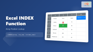
Excel INDEX Function: Complete Guide to Array Position Lookup with Practical Examples
The Excel INDEX function is one of the most powerful and versatile lookup functions available in Microsoft Excel. Unlike other...

Excel TABLE Function: Complete Guide to Structured Data Management and Advanced Formulas
What is the Excel TABLE Function? The Excel TABLE function is a powerful feature that converts regular cell ranges into...
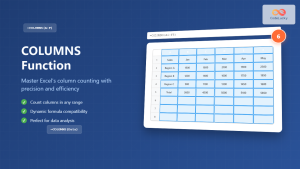
Excel COLUMNS Function: Master Column Counting with Practical Examples
The Excel COLUMNS function is a powerful built-in tool that counts the number of columns in a specified range or...

Excel FIND Function: Complete Guide to Text Position Finding in Spreadsheets
The Excel FIND function is a powerful text manipulation tool that helps you locate the position of specific characters or...

Excel DGET Function: Complete Guide to Database Single Value Extraction
What is the Excel DGET Function? The DGET function in Microsoft Excel is a powerful database function designed to extract...

Excel ISNA Function: Complete Guide to NA Value Detection and Error Handling
What is the Excel ISNA Function? The ISNA function in Microsoft Excel is a powerful logical function designed to detect...
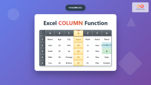
Excel COLUMN Function: Complete Guide to Column Number References
The Excel COLUMN function is a fundamental lookup and reference function that returns the column number of a specified cell...

Excel IF Function: Complete Guide to Conditional Logic Formulas
The Excel IF function is one of the most fundamental and powerful logical functions in Microsoft Excel, enabling users to...