Excel MATCH Function: Complete Position Finding Formula Guide with Examples

The MATCH function in Microsoft Excel is a powerful lookup formula that finds the relative position of a value within an array or range. Unlike VLOOKUP or INDEX, MATCH doesn’t return the actual value—it returns the position number where your lookup value is found.

This comprehensive guide will teach you everything about the MATCH function, from basic syntax to advanced applications that will transform how you handle data analysis in Excel.

What is the Excel MATCH Function?

The MATCH function searches for a specified value in a range of cells and returns the relative position of that value. Think of it as Excel’s way of answering “Where is this item located?” rather than “What is this item?”

The function is particularly useful when combined with other functions like INDEX, creating dynamic lookup formulas that are more flexible than traditional VLOOKUP functions.

MATCH Function Syntax

The MATCH function follows this syntax structure:

=MATCH(lookup_value, lookup_array, [match_type])

Parameters Explained:

• lookup_value (Required): The value you want to find the position of
• lookup_array (Required): The range of cells where you want to search
• match_type (Optional): Specifies how Excel matches the lookup_value

Match Type Options:

• 1 or TRUE (Default): Finds the largest value less than or equal to lookup_value (requires sorted data in ascending order)
• 0 or FALSE: Finds exact match only
• -1: Finds the smallest value greater than or equal to lookup_value (requires sorted data in descending order)

Basic MATCH Function Examples

Example 1: Finding Exact Position

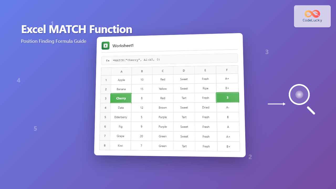
Suppose you have a list of fruits in cells A1:A5:

• A1: Apple
• A2: Banana
• A3: Cherry
• A4: Date
• A5: Elderberry

To find the position of “Cherry”, use:

=MATCH("Cherry", A1:A5, 0)

This returns 3 because Cherry is in the third position of the range.

Example 2: Using Cell References

Instead of typing the lookup value directly, reference a cell:

=MATCH(D1, A1:A5, 0)

Where D1 contains the value you’re searching for.

Example 3: Approximate Match with Sorted Data

For numerical data sorted in ascending order (B1:B10 contains values 10, 20, 30, 40, 50…):

=MATCH(35, B1:B10, 1)

This returns the position of the largest value that’s less than or equal to 35, which would be position 3 (value 30).

Advanced MATCH Function Techniques

Using MATCH with Wildcards

When match_type is 0, you can use wildcards for partial matching:

• ? (question mark): Represents any single character
• * (asterisk): Represents any sequence of characters

=MATCH("App*", A1:A5, 0)

This finds the first cell that starts with “App”, returning the position of “Apple”.

Two-Way Lookup with MATCH

Combine two MATCH functions to find both row and column positions:

=INDEX(B2:E10, MATCH("Product A", A2:A10, 0), MATCH("Q2", B1:E1, 0))

This formula finds “Product A” in the first column and “Q2” in the first row, then returns the intersecting value.

Finding Last Occurrence

To find the last occurrence of a value in a range, use an array formula:

=LOOKUP(2, 1/(A1:A10="SearchValue"), ROW(A1:A10))

MATCH Function Error Handling

Common Errors and Solutions

#N/A Error: Occurs when no match is found. Wrap your MATCH function with IFERROR:

=IFERROR(MATCH("Value", A1:A10, 0), "Not Found")

#VALUE! Error: Usually happens with data type mismatches. Ensure your lookup_value and lookup_array contain compatible data types.

Best Practices for Error Prevention

• Always use match_type 0 for exact matches unless you specifically need approximate matching
• Trim spaces from text data using the TRIM function
• Use IFERROR or IF(ISERROR()) to handle cases where no match exists
• Ensure data types match between lookup_value and the lookup_array

MATCH vs Other Lookup Functions

MATCH vs VLOOKUP

• MATCH: Returns position number, works with any orientation
• VLOOKUP: Returns actual values, only works left-to-right

MATCH vs FIND/SEARCH

• MATCH: Finds position in arrays/ranges
• FIND/SEARCH: Finds character position within text strings

Real-World Applications

Dynamic Dashboard Creation

Use MATCH to create dynamic charts and dashboards where users can select different time periods or categories, and the formulas automatically adjust to show relevant data.

Data Validation Lists

Combine MATCH with data validation to ensure users only enter values that exist in your reference lists.

Performance Tracking

Find employee rankings, product performance positions, or any scenario where you need to know relative standings rather than absolute values.

Performance Optimization Tips

Sorting for Speed

When using approximate match (match_type 1 or -1), ensure your data is properly sorted. This allows Excel to use more efficient search algorithms.

Range Size Considerations

Limit your lookup_array to the smallest possible range. Searching through entire columns (A:A) is slower than specific ranges (A1:A1000).

Volatile Function Alternatives

MATCH is generally more efficient than volatile functions like INDIRECT when used in lookup scenarios.

Troubleshooting Common Issues

Case Sensitivity

MATCH is not case-sensitive by default. “apple” will match “Apple”. If you need case-sensitive matching, combine with EXACT function:

=MATCH(TRUE, EXACT("apple", A1:A10), 0)

Leading/Trailing Spaces

Hidden spaces often cause match failures. Clean your data with:

=MATCH(TRIM("Value"), A1:A10, 0)

Number Format Mismatches

Numbers stored as text won’t match actual numbers. Use VALUE function to convert:

=MATCH(VALUE(D1), A1:A10, 0)

Advanced Array Formulas with MATCH

Multiple Criteria Matching

Find positions based on multiple conditions using array formulas:

=MATCH(1, (A1:A10="Criteria1")*(B1:B10="Criteria2"), 0)

This finds the first row where both conditions are met.

Closest Value Matching

Find the position of the value closest to your lookup value:

=MATCH(MIN(ABS(A1:A10-SearchValue)), ABS(A1:A10-SearchValue), 0)

Integration with Modern Excel Features

Dynamic Arrays and Spill Ranges

In Excel 365, MATCH works seamlessly with dynamic arrays and spill ranges, automatically adjusting as your data expands.

Power Query Integration

While Power Query has its own matching capabilities, MATCH remains valuable for dynamic formulas that update automatically with data changes.

Conclusion

The MATCH function is an essential tool in Excel’s formula arsenal, offering precise position-finding capabilities that complement other lookup functions perfectly. By mastering MATCH, you unlock the ability to create more dynamic, flexible, and powerful spreadsheet solutions.

Whether you’re building complex dashboards, performing data analysis, or creating user-friendly interfaces, the MATCH function provides the positional intelligence your formulas need to adapt and respond to changing data conditions.

Practice these techniques with your own data sets, and you’ll quickly discover how MATCH can transform static spreadsheets into dynamic, intelligent tools that grow with your needs.