The VLOOKUP function is one of Excel’s most powerful and frequently used lookup functions, enabling users to search for specific data within large datasets efficiently. This comprehensive guide will walk you through everything you need to know about VLOOKUP, from basic syntax to advanced applications.
What is VLOOKUP Function?
VLOOKUP (Vertical Lookup) is an Excel function that searches for a value in the first column of a table and returns a corresponding value from a specified column in the same row. The “V” in VLOOKUP stands for “vertical” because it searches vertically down the first column of your data range.
This function is particularly useful when working with large databases, customer lists, inventory management, or any scenario where you need to quickly find related information based on a unique identifier.
VLOOKUP Syntax and Arguments
The basic syntax of the VLOOKUP function is:
=VLOOKUP(lookup_value, table_array, col_index_num, [range_lookup])Breaking Down Each Argument:
lookup_value: This is the value you want to search for. It can be a cell reference, text string, number, or logical value. The function will search for this value in the first column of your table array.
table_array: This represents the range of cells containing your data table. The lookup value must be in the first column of this range, and the function will return data from other columns within this range.
col_index_num: This is the column number from which you want to return a value. The first column in your table array is column 1, the second is column 2, and so on.
range_lookup: This optional argument determines the type of match. Use FALSE or 0 for exact match, and TRUE or 1 for approximate match. If omitted, Excel assumes TRUE.
Basic VLOOKUP Examples
Example 1: Employee Salary Lookup
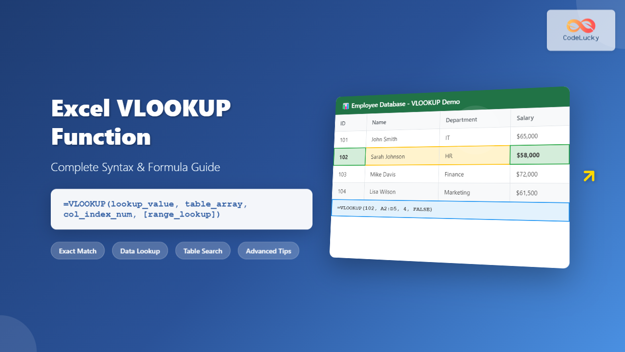
Consider a simple employee database with the following structure:
| Employee ID | Name | Department | Salary |
|---|---|---|---|
| 101 | John Smith | IT | $65,000 |
| 102 | Sarah Johnson | HR | $58,000 |
| 103 | Mike Davis | Finance | $72,000 |
To find John Smith’s salary using his Employee ID (101), you would use:
=VLOOKUP(101, A2:D4, 4, FALSE)This formula searches for “101” in the first column (A2:A4), finds it in row 2, and returns the value from the 4th column (salary) of that row.
Example 2: Product Price Lookup
For a product catalog where you want to find prices based on product codes:
=VLOOKUP("PROD001", Products!A:C, 3, FALSE)This searches for “PROD001” in column A of the Products sheet and returns the price from column C.
Exact Match vs Approximate Match
Exact Match (FALSE or 0)
When you set the range_lookup parameter to FALSE, VLOOKUP searches for an exact match. This is the most commonly used option and is recommended for:
- Employee IDs, product codes, or customer numbers
- Text values that must match precisely
- Any scenario where you need exact correspondence
Approximate Match (TRUE or 1)
When set to TRUE, VLOOKUP finds the closest match that is less than or equal to the lookup value. This requires your data to be sorted in ascending order and is useful for:
- Grade scales (finding letter grades based on numeric scores)
- Commission tiers
- Tax brackets
Advanced VLOOKUP Techniques
Using VLOOKUP with Named Ranges
You can make your formulas more readable by using named ranges:
=VLOOKUP(A2, EmployeeData, 3, FALSE)Where “EmployeeData” is a named range containing your lookup table.
Dynamic Column Index with MATCH Function
Instead of hardcoding column numbers, use the MATCH function to make your formula more flexible:
=VLOOKUP(A2, DataTable, MATCH("Salary", DataTable[#Headers], 0), FALSE)This automatically finds the column number for “Salary” header.
Handling Errors with IFERROR
Wrap your VLOOKUP in an IFERROR function to handle cases where the lookup value isn’t found:
=IFERROR(VLOOKUP(A2, DataTable, 3, FALSE), "Not Found")Common VLOOKUP Errors and Solutions
#N/A Error
This occurs when VLOOKUP cannot find the lookup value. Common causes include:
- Typos in the lookup value
- Extra spaces or different formatting
- The lookup value doesn’t exist in the first column
Solution: Use TRIM function to remove extra spaces, or IFERROR to handle missing values gracefully.
#REF! Error
This happens when the col_index_num is greater than the number of columns in your table_array.
Solution: Verify that your column index number doesn’t exceed the actual number of columns in your range.
#VALUE! Error
This occurs when col_index_num is less than 1.
Solution: Ensure your column index number is at least 1.
VLOOKUP Best Practices
Data Organization
Structure your data with the lookup column as the leftmost column in your table array. VLOOKUP can only search to the right, so the data you want to retrieve must be in columns to the right of your lookup column.
Use Absolute References
When copying formulas, use absolute references for your table array:
=VLOOKUP(A2, $B$2:$E$100, 3, FALSE)Optimize Performance
For large datasets, consider using exact match (FALSE) as it’s generally faster than approximate match. Also, limit your table array to only the necessary data range.
Alternatives to VLOOKUP
INDEX and MATCH Combination
This combination is more flexible than VLOOKUP as it can lookup values to the left:
=INDEX(C2:C100, MATCH(A2, B2:B100, 0))XLOOKUP Function
Available in newer Excel versions, XLOOKUP is more powerful and user-friendly:
=XLOOKUP(A2, B2:B100, C2:C100)Real-World Applications
Inventory Management
Use VLOOKUP to find product details, current stock levels, or reorder points based on product codes.
Customer Relationship Management
Look up customer information, purchase history, or contact details using customer IDs.
Financial Analysis
Retrieve account balances, transaction details, or budget allocations based on account numbers.
Human Resources
Find employee information, salary details, or department assignments using employee IDs.
Tips for Mastering VLOOKUP
Start with simple examples and gradually work your way up to more complex scenarios. Practice with different data types and always test your formulas with known values to ensure accuracy.
Remember that VLOOKUP is case-insensitive for text values, which can be both helpful and problematic depending on your needs. If case sensitivity is important, consider using exact match with additional text functions.
Keep your data clean and consistent. Remove extra spaces, ensure consistent formatting, and avoid merged cells in your lookup tables for best results.
Conclusion
VLOOKUP is an essential Excel function that significantly improves data analysis efficiency. By understanding its syntax, mastering both exact and approximate match options, and following best practices, you can handle complex data lookup tasks with confidence. Whether you’re managing inventory, analyzing sales data, or organizing employee information, VLOOKUP will become an invaluable tool in your Excel toolkit.
As you become more comfortable with VLOOKUP, consider exploring its alternatives like INDEX-MATCH or XLOOKUP for even more powerful data manipulation capabilities. The key to mastering any Excel function is consistent practice with real-world data scenarios.

