Excel IMPLICIT Intersection: Complete Guide to Legacy Array Formula Behavior

Excel’s IMPLICIT intersection is a critical concept that bridges the gap between traditional single-cell formulas and modern dynamic array formulas. Understanding this behavior is essential for Excel users working with legacy spreadsheets or maintaining backward compatibility in their workbooks.

What is Excel IMPLICIT Intersection?

IMPLICIT intersection is Excel’s automatic mechanism that converts array formulas into single-value results when entered in a single cell. This operator (@) appears automatically when Excel detects that a formula would normally return multiple values but is constrained to a single cell output.

When you see the @ symbol prefixing your formula in the formula bar, Excel is telling you that it has applied implicit intersection to return only one value from what could be a multi-value array result.

How IMPLICIT Intersection Works

The IMPLICIT operator follows specific rules to determine which value to return from an array:

Row-Based Intersection

When a formula returns multiple values in the same row as the formula cell, Excel returns the value from the column that matches the formula’s position. For example, if your formula is in cell C5 and returns values across columns A through E in row 5, Excel will return the value from column C.

Column-Based Intersection

Similarly, when a formula returns multiple values in the same column as the formula cell, Excel returns the value from the row that matches the formula’s position.

Single Value Return

If the intersection results in exactly one value, that value is returned. If no intersection exists or multiple intersections occur, Excel typically returns the first value from the array.

Common Scenarios Where IMPLICIT Intersection Occurs

Legacy VLOOKUP and INDEX/MATCH Formulas

Traditional lookup functions often trigger implicit intersection when they reference entire columns or large ranges. For instance:

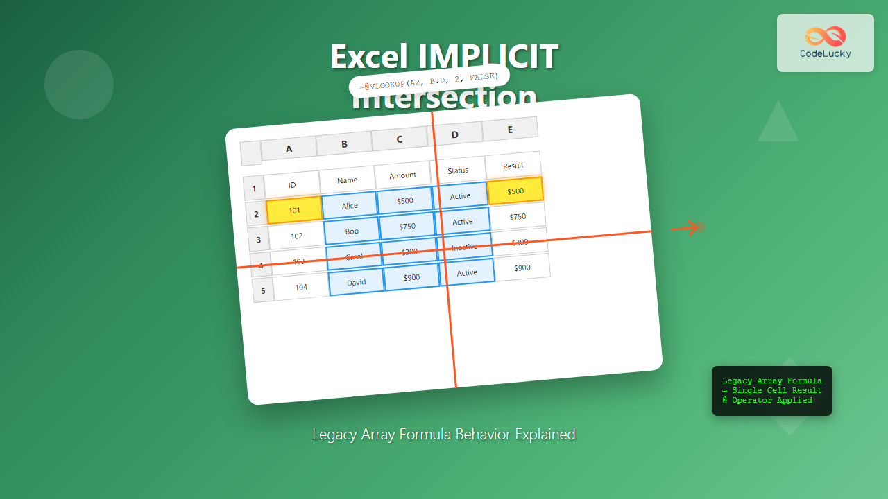
=VLOOKUP(A2, B:D, 2, FALSE)

This formula might display as =@VLOOKUP(A2, B:D, 2, FALSE) in newer Excel versions, indicating that Excel is applying implicit intersection to ensure a single result.

Range References in Arithmetic Operations

When you reference entire ranges in calculations, Excel may apply implicit intersection:

=A:A * B:B

This becomes =@A:A * @B:B, returning only the result for the current row.

Function Results with Multiple Outputs

Functions that naturally return arrays, such as FILTER, SORT, or UNIQUE, will show the implicit intersection operator when entered in a single cell that cannot accommodate the full array result.

Differences Between Legacy and Modern Array Behavior

Pre-Dynamic Array Excel Versions

In older Excel versions (prior to Office 365), array formulas required manual entry using Ctrl+Shift+Enter, creating “CSE formulas” surrounded by curly braces {}. These formulas would:

• Process entire arrays but return single values through implicit intersection
• Require specific array formula syntax
• Show curly braces in the formula bar when properly entered
• Limit spill behavior to pre-selected ranges

Modern Dynamic Array Excel

Current Excel versions with dynamic arrays automatically:

• Spill results across multiple cells when space allows
• Apply implicit intersection only when necessary
• Show the @ operator to indicate intersection
• Allow seamless transition between single and multiple results

Practical Examples of IMPLICIT Intersection

Example 1: SUM with Range References

Consider this formula in cell D5:

=SUM(A:A)

Excel might display this as =@SUM(A:A), but since SUM inherently returns a single value, the implicit intersection doesn’t change the result.

Example 2: Array Formula Conversion

If you have a formula that returns multiple values:

=IF(A1:A10>5, A1:A10, "")

In a single cell, this becomes =@IF(A1:A10>5, A1:A10, ""), returning only the result corresponding to your formula’s row position.

Example 3: Lookup Function Behavior

A complex lookup might appear as:

=@INDEX(Data[Amount], MATCH(A2, Data[ID], 0))

The implicit intersection ensures that even if the INDEX function could return multiple values, only one result appears in your cell.

Managing IMPLICIT Intersection in Your Workbooks

When to Embrace IMPLICIT Intersection

IMPLICIT intersection is beneficial when you:

• Need to maintain compatibility with older Excel versions
• Want single-value results from potentially multi-value formulas
• Are working with existing legacy formulas that rely on this behavior
• Need to prevent accidental spilling in constrained layouts

When to Override IMPLICIT Intersection

You might want to force array behavior by:

• Manually removing the @ operator to allow spilling
• Using array-specific functions like FILTER or SORT
• Selecting a range before entering the formula to define the output area
• Wrapping formulas in functions that naturally handle arrays

Troubleshooting IMPLICIT Intersection Issues

Unexpected Single Results

If your formula returns only one value when you expected multiple results, check for the @ operator. Remove it to allow the formula to spill across multiple cells, provided there’s adequate space.

Compatibility Problems

When sharing workbooks between different Excel versions, implicit intersection can cause formulas to behave differently. Test your workbooks across different Excel versions to ensure consistent behavior.

Performance Considerations

Implicit intersection can impact performance when applied to large ranges. Consider using more specific range references or optimized functions when dealing with extensive datasets.

Best Practices for IMPLICIT Intersection

Documentation and Comments

Always document formulas that rely on implicit intersection behavior, especially in shared workbooks. Use cell comments to explain the expected behavior and any version-specific considerations.

Testing Across Versions

Regularly test your workbooks in different Excel versions to ensure that implicit intersection behaves as expected. This is particularly important for workbooks used across organizations with varying Excel installations.

Explicit Range Definition

When possible, use explicit range references rather than entire column references to make your intentions clear and improve performance.

Advanced Techniques with IMPLICIT Intersection

Combining with Dynamic Arrays

You can strategically use implicit intersection alongside dynamic array functions to create sophisticated formulas that adapt to different contexts:

=@FILTER(Data[Amount], Data[Category]=E2)

This formula will return only the first matching result in a single cell, while the same formula without the @ operator would spill all matching results.

Conditional Array Processing

Use implicit intersection to process arrays conditionally:

=@IF(ROWS(A:A)>1000, SUMMARIZE(A:A), A:A)

This approach allows your formulas to adapt their behavior based on data size or other conditions.

Future Considerations

As Excel continues to evolve, understanding implicit intersection becomes increasingly important for:

• Maintaining legacy workbook functionality
• Ensuring smooth transitions between Excel versions
• Optimizing formula performance in mixed environments
• Developing robust, version-independent solutions

Excel’s IMPLICIT intersection represents a thoughtful approach to backward compatibility while enabling modern array functionality. By mastering this concept, you can create more reliable, efficient, and compatible Excel solutions that work seamlessly across different versions and use cases.

Whether you’re maintaining existing spreadsheets or developing new solutions, understanding when and how Excel applies implicit intersection will help you write better formulas and avoid unexpected results in your data analysis workflows.