Excel’s dynamic array formulas revolutionized spreadsheet calculations by automatically expanding results across multiple cells. These powerful functions eliminate the need for complex array formulas and make data analysis more intuitive and efficient.
What Are Dynamic Array Formulas?
Dynamic array formulas are Excel functions that return multiple values to a range of cells automatically. Unlike traditional formulas that return single values, these functions create spill ranges – areas where results automatically expand or contract based on the data.
Key characteristics of dynamic arrays include:
- Automatic result expansion across multiple cells
- Single formula entry that populates multiple outputs
- Dynamic resizing when source data changes
- Enhanced calculation performance compared to array formulas
Understanding Spill Ranges
A spill range refers to the area where dynamic array results automatically populate. When you enter a dynamic array formula, Excel calculates all results and “spills” them into adjacent cells.
Spill Range Behavior
Spill ranges exhibit several important behaviors:
- Automatic expansion: Results fill as many cells as needed
- Dynamic resizing: Range adjusts when data changes
- Overwrite protection: Formulas won’t spill into occupied cells
- Reference consistency: Entire spill range updates simultaneously
Spill Range Reference Operator (#)
The hash symbol (#) is the spill range reference operator that refers to the entire spilled array. For example, if cell A1 contains a dynamic array formula, A1# references the complete spill range.
=SORT(A1#)  // References entire spill range from A1
=SUM(B2#)   // Sums all values in spill range starting at B2
Complete List of Dynamic Array Functions
Excel includes 14 dynamic array functions, each serving specific data manipulation purposes:
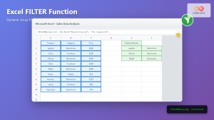
1. FILTER Function
The FILTER function extracts data that meets specified criteria.
Syntax: =FILTER(array, include, [if_empty])
=FILTER(A2:D10, C2:C10>100)
// Returns rows where column C values exceed 100
2. SORT Function
SORT arranges data in ascending or descending order.
Syntax: =SORT(array, [sort_index], [sort_order], [by_col])
=SORT(A1:C10, 2, -1)
// Sorts by second column in descending order
3. SORTBY Function
SORTBY sorts data based on corresponding values in other arrays.
Syntax: =SORTBY(array, by_array1, [sort_order1], ...)
=SORTBY(A2:B10, C2:C10, -1)
// Sorts A2:B10 based on C2:C10 values in descending order
4. UNIQUE Function
UNIQUE returns distinct values from a list or range.
Syntax: =UNIQUE(array, [by_col], [exactly_once])
=UNIQUE(A2:A100)
// Returns unique values from range A2:A100
5. SEQUENCE Function
SEQUENCE generates sequential numbers in rows and columns.
Syntax: =SEQUENCE(rows, [columns], [start], [step])
=SEQUENCE(10, 1, 5, 2)
// Creates 10 numbers starting from 5, incrementing by 2
6. RANDARRAY Function
RANDARRAY generates arrays of random numbers.
Syntax: =RANDARRAY([rows], [columns], [min], [max], [whole_number])
=RANDARRAY(5, 3, 1, 100, TRUE)
// Creates 5x3 array of random whole numbers between 1-100
7. XLOOKUP Function
XLOOKUP is an enhanced lookup function replacing VLOOKUP and HLOOKUP.
Syntax: =XLOOKUP(lookup_value, lookup_array, return_array, [if_not_found], [match_mode], [search_mode])
=XLOOKUP(E2, A2:A100, B2:D100)
// Returns multiple columns for matching lookup value
8. XMATCH Function
XMATCH returns the relative position of items in an array.
Syntax: =XMATCH(lookup_value, lookup_array, [match_mode], [search_mode])
=XMATCH("Product A", A2:A50, 0)
// Returns position of exact match for "Product A"
9. TRANSPOSE Function (Enhanced)
TRANSPOSE converts rows to columns and vice versa with dynamic array support.
Syntax: =TRANSPOSE(array)
=TRANSPOSE(A1:E1)
// Converts horizontal range to vertical
10. MMULT Function (Enhanced)
MMULT performs matrix multiplication with dynamic arrays.
Syntax: =MMULT(array1, array2)
11. FREQUENCY Function (Enhanced)
FREQUENCY calculates frequency distributions dynamically.
Syntax: =FREQUENCY(data_array, bins_array)
12. MODE.SNGL Function (Enhanced)
Returns the most frequently occurring value with dynamic array support.
13. SUMPRODUCT Function (Enhanced)
Enhanced SUMPRODUCT works seamlessly with dynamic arrays.
14. MINIFS/MAXIFS Functions (Enhanced)
These functions now support dynamic array criteria ranges.
Advanced Spill Range Techniques
Combining Multiple Dynamic Functions
Dynamic array functions can be nested and combined for powerful data manipulation:
=SORT(UNIQUE(FILTER(A2:C100, B2:B100="Active")), 1)
// Filters active records, finds unique values, then sorts
Using Spill Ranges in Calculations
Reference entire spill ranges in other formulas using the # operator:
=SUM(FILTER(B2:B100, A2:A100="Sales")#)
// Sums the entire filtered result
Creating Dynamic Charts
Use dynamic array formulas as chart data sources for automatically updating visualizations:
- Create dynamic array formula
- Select the spill range
- Insert chart
- Chart updates automatically when data changes
Common Spill Errors and Solutions
#SPILL! Error
The #SPILL! error occurs when Excel cannot complete the spill operation:
- Blocked cells: Clear cells in the intended spill range
- Merged cells: Unmerge cells in the spill area
- Table interference: Ensure spill range doesn’t conflict with tables
Performance Optimization
Optimize dynamic array performance with these techniques:
- Use specific ranges instead of entire columns
- Limit nested function complexity
- Consider calculation mode settings
- Use structured references in tables
Practical Examples and Use Cases
Data Analysis Dashboard
// Top 10 sales by region
=SORT(FILTER(Sales_Data, Region="North"), 3, -1)

// Unique customer list
=SORT(UNIQUE(Customer_Column))

// Monthly summary
=SUMIFS(Amount#, Month#, SEQUENCE(12))
Report Generation
// Dynamic report headers
=TRANSPOSE(UNIQUE(Category_Range))

// Filtered results by date range
=FILTER(Data_Range, (Date_Column>=StartDate)*(Date_Column<=EndDate))
Best Practices for Dynamic Arrays
Follow these best practices for optimal dynamic array implementation:
- Plan spill ranges: Ensure adequate space for results
- Use meaningful names: Apply defined names to dynamic ranges
- Document formulas: Add comments explaining complex combinations
- Test with varying data sizes: Verify formulas work with different data volumes
- Consider calculation impact: Monitor performance with large datasets
Conclusion
Excel's dynamic array formulas represent a significant advancement in spreadsheet functionality. By mastering spill ranges and the 14 dynamic functions, you can create more efficient, maintainable, and powerful data analysis solutions. These tools eliminate many traditional Excel limitations while providing unprecedented flexibility for data manipulation and analysis.
Start implementing dynamic arrays in your workflows to experience improved productivity and simplified formula management. As your proficiency grows, explore advanced combinations and techniques to unlock the full potential of Excel's dynamic array capabilities.
Related Posts
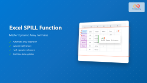
Excel SPILL Function: Complete Guide to Array Spill Range Commands
What is the Excel SPILL Function? The Excel SPILL function is a powerful dynamic array feature introduced in Microsoft Excel...

Excel OFFSET Function: Dynamic Reference Formula for Advanced Data Management
The Excel OFFSET function is one of the most powerful yet underutilized tools for creating dynamic references in spreadsheets. This...
Excel FILTER Function: Complete Guide to Dynamic Array Filtering
The Excel FILTER function is one of the most powerful dynamic array functions introduced in Excel 365 and Excel 2021....
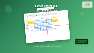
Excel IMPLICIT Intersection: Complete Guide to Legacy Array Formula Behavior
Excel's IMPLICIT intersection is a critical concept that bridges the gap between traditional single-cell formulas and modern dynamic array formulas....

Excel TABLE Function: Complete Guide to Structured Data Management and Advanced Formulas
What is the Excel TABLE Function? The Excel TABLE function is a powerful feature that converts regular cell ranges into...
Excel AREAS Function: Complete Guide to Count Reference Areas in Formulas
The Excel AREAS function is a powerful reference function that counts the number of areas (separate ranges) within a given...
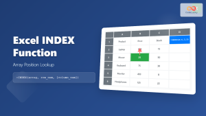
Excel INDEX Function: Complete Guide to Array Position Lookup with Practical Examples
The Excel INDEX function is one of the most powerful and versatile lookup functions available in Microsoft Excel. Unlike other...

Excel COLUMNS Function: Master Column Counting with Practical Examples
The Excel COLUMNS function is a powerful built-in tool that counts the number of columns in a specified range or...

Excel CHOOSE Function: Dynamic Value Selection Made Simple
The Excel CHOOSE function is a powerful lookup and reference function that allows you to select and return a specific...
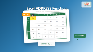
Excel ADDRESS Function: Complete Guide to Dynamic Cell Reference Creation
The Excel ADDRESS function is a powerful text function that creates cell references as text strings based on row and...

Excel RANDARRAY Function: Complete Guide to Dynamic Random Array Generation
What is the Excel RANDARRAY Function? The RANDARRAY function is a powerful dynamic array function in Microsoft Excel that generates...

Excel COLUMN Function: Complete Guide to Column Number References
The Excel COLUMN function is a fundamental lookup and reference function that returns the column number of a specified cell...