The Excel FILTER function is one of the most powerful dynamic array functions introduced in Excel 365 and Excel 2021. This revolutionary function allows you to extract specific data from a range or array based on criteria you define, automatically spilling results into adjacent cells without the need for complex formulas or manual filtering.
What is the Excel FILTER Function?
The FILTER function extracts data that meets specific criteria from a source array or range. Unlike traditional filtering methods that hide rows, the FILTER function creates a new dynamic array containing only the data that matches your conditions. This makes it incredibly useful for creating dashboards, reports, and dynamic data analysis.
Key Benefits of Using FILTER Function
- Dynamic Results: Automatically updates when source data changes
- No Manual Intervention: Eliminates the need to manually adjust filters
- Multiple Criteria: Supports complex filtering conditions
- Preserves Original Data: Creates filtered copies without affecting source data
- Formula-Based: Can be combined with other functions for advanced operations
FILTER Function Syntax
The FILTER function follows this syntax:
=FILTER(array, include, [if_empty])
Parameters Explained
- array (required): The range or array you want to filter
- include (required): A Boolean array that determines which rows or columns to include
- if_empty (optional): The value to return if no data meets the criteria
Basic FILTER Function Examples
Example 1: Simple Text Filtering
Suppose you have a list of products and want to filter only those in the “Electronics” category:
=FILTER(A2:C10, B2:B10="Electronics")
This formula filters the range A2:C10 and returns only rows where column B contains “Electronics”.
Example 2: Numeric Filtering
To filter sales data for amounts greater than $1000:
=FILTER(A2:D20, D2:D20>1000)
This returns all rows where the value in column D exceeds 1000.
Example 3: Using the if_empty Parameter
To display a custom message when no data matches your criteria:
=FILTER(A2:C10, B2:B10="Gadgets", "No gadgets found")
If no rows contain “Gadgets” in column B, the formula returns “No gadgets found” instead of an error.
Advanced FILTER Function Techniques
Multiple Criteria with AND Logic
To filter data that meets multiple conditions simultaneously, use the multiplication operator (*) or the AND function:
=FILTER(A2:D20, (B2:B20="Electronics") * (D2:D20>500))
This formula returns rows where the category is “Electronics” AND the value is greater than 500.
Multiple Criteria with OR Logic
For OR conditions, use the addition operator (+) or the OR function:
=FILTER(A2:D20, (B2:B20="Electronics") + (B2:B20="Computers"))
This returns rows where the category is either “Electronics” OR “Computers”.
Text-Based Filtering with Wildcards
Use functions like SEARCH or FIND for partial text matching:
=FILTER(A2:C20, ISNUMBER(SEARCH("Apple", A2:A20)))
This filters rows containing “Apple” anywhere in column A, regardless of case.
Combining FILTER with Other Functions
FILTER with SORT
Create filtered and sorted results in one formula:
=SORT(FILTER(A2:D20, C2:C20>100), 4, 1)
This filters data where column C is greater than 100, then sorts by column 4 in ascending order.
FILTER with UNIQUE
Get unique values from filtered results:
=UNIQUE(FILTER(A2:A20, B2:B20="Active"))
This returns unique values from column A where column B equals “Active”.
FILTER with SUM
Calculate totals from filtered data:
=SUM(FILTER(D2:D20, B2:B20="Sales"))
This sums values in column D where column B contains “Sales”.
Common FILTER Function Errors and Solutions
#CALC! Error
This error occurs when the array and include parameters have different dimensions. Ensure both ranges have the same number of rows.
Incorrect: =FILTER(A2:C10, B2:B15="Test")
Correct: =FILTER(A2:C10, B2:B10="Test")
#VALUE! Error
This happens when the include parameter doesn’t return Boolean values. Check your criteria logic.
Empty Results
When no data matches your criteria, use the if_empty parameter to display a meaningful message instead of an error.
Performance Tips for FILTER Function
Optimize Large Datasets
- Use structured table references instead of static ranges
- Limit the array size to necessary columns only
- Consider using INDEX and MATCH for single-value lookups
Memory Management
Dynamic arrays can consume significant memory with large datasets. Monitor your workbook’s performance and consider breaking down complex FILTER operations into smaller chunks.
Real-World Applications
Sales Dashboard
Create dynamic sales reports that automatically update:
=FILTER(SalesData, (SalesData[Date]>=StartDate) * (SalesData[Date]<=EndDate) * (SalesData[Region]=SelectedRegion))
Inventory Management
Track low-stock items automatically:
=FILTER(Inventory, Inventory[Stock]
Employee Records
Filter employee data by department and status:
=FILTER(Employees, (Employees[Department]="IT") * (Employees[Status]="Active"))
FILTER vs Traditional Filtering Methods
Advantages Over AutoFilter
- Formula-based: Results update automatically with data changes
- Multiple instances: Create several filtered views simultaneously
- Integration: Easily combine with other functions and formulas
- Preservation: Original data remains unaltered and visible
Comparison with Advanced Filter
While Advanced Filter offers more complex criteria options, the FILTER function provides:
- Simpler syntax for most common scenarios
- Dynamic results that auto-refresh
- Better integration with modern Excel features
- No need for separate criteria ranges
Browser and Version Compatibility
The FILTER function is available in:
- Excel 365 (all platforms)
- Excel 2021 (Windows and Mac)
- Excel for the web
- Excel mobile apps
Note: The function is not available in Excel 2019 or earlier versions. Users with older versions should consider upgrading or using alternative methods like Advanced Filter or pivot tables.
Best Practices and Tips
Formula Design
- Always use the if_empty parameter to handle scenarios with no matching data
- Test your criteria logic with small datasets before applying to large ranges
- Use meaningful variable names in structured references
- Document complex FILTER formulas with comments
Error Prevention
- Ensure array and criteria ranges have matching dimensions
- Use absolute references ($) when copying formulas
- Validate data types in your criteria
- Test edge cases like empty cells or special characters
Troubleshooting Common Issues
Formula Not Updating
If your FILTER results don't update when source data changes:
- Check if calculation mode is set to Automatic
- Press Ctrl+Alt+F9 to force recalculation
- Verify that source data is properly formatted as a table or range
Spill Errors
When FILTER results can't display due to occupied cells:
- Clear cells in the spill range
- Move the FILTER formula to a different location
- Use the spill range operator (#) to reference the entire result
Conclusion
The Excel FILTER function represents a significant advancement in spreadsheet data manipulation, offering dynamic, formula-based filtering that automatically adapts to changing data. By mastering this function and its various applications, you can create more responsive and efficient spreadsheets that require less manual maintenance.
Whether you're building dashboards, analyzing sales data, or managing inventory, the FILTER function provides the flexibility and power needed for modern data analysis tasks. Combined with other dynamic array functions like SORT, UNIQUE, and XLOOKUP, it forms the foundation of next-generation Excel formulas.
Start implementing FILTER in your workflows today, and experience the efficiency gains that come with truly dynamic data filtering in Excel.
Related Posts
Excel Dynamic Array Formulas: Complete Spill Range Syntax and Functions Guide
Excel's dynamic array formulas revolutionized spreadsheet calculations by automatically expanding results across multiple cells. These powerful functions eliminate the need...
Excel SORT Function: Complete Guide to Dynamic Array Sorting Formula
The Excel SORT function is a powerful dynamic array formula introduced in Excel 365 that allows you to sort data...
Excel SPILL Function: Complete Guide to Array Spill Range Commands
What is the Excel SPILL Function? The Excel SPILL function is a powerful dynamic array feature introduced in Microsoft Excel...

Excel TABLE Function: Complete Guide to Structured Data Management and Advanced Formulas
What is the Excel TABLE Function? The Excel TABLE function is a powerful feature that converts regular cell ranges into...

Excel SORTBY Function: Master Dynamic Array Sorting with Advanced Custom Commands
The Excel SORTBY function revolutionizes how we handle data sorting by providing dynamic array functionality that automatically updates when source...
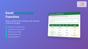
Excel AVERAGEIFS Function: Master Multiple Criteria Calculations
The AVERAGEIFS function in Microsoft Excel is a powerful statistical tool that enables users to calculate the average of cells...
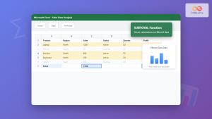
Excel SUBTOTAL Function: Complete Guide to Filtered Data Calculations
The Excel SUBTOTAL function is one of the most powerful yet underutilized functions in Microsoft Excel. Unlike standard aggregation functions...

Excel OFFSET Function: Dynamic Reference Formula for Advanced Data Management
The Excel OFFSET function is one of the most powerful yet underutilized tools for creating dynamic references in spreadsheets. This...
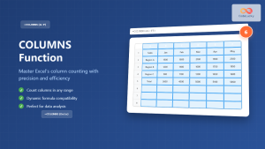
Excel COLUMNS Function: Master Column Counting with Practical Examples
The Excel COLUMNS function is a powerful built-in tool that counts the number of columns in a specified range or...
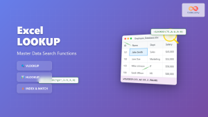
Excel LOOKUP Function: Complete Guide to Basic Search Commands and Advanced Techniques
The LOOKUP function in Microsoft Excel is a powerful search tool that allows you to find specific values within your...

Excel XLOOKUP Function: Complete Guide to Modern Lookup Formulas
Excel's XLOOKUP function represents a revolutionary advancement in spreadsheet lookup capabilities, offering a modern alternative to traditional VLOOKUP and HLOOKUP...

Excel UNIQUE Function: Extract Unique Values with Advanced Formulas
The Excel UNIQUE function is a powerful dynamic array formula introduced in Excel 365 and Excel 2021 that allows you...