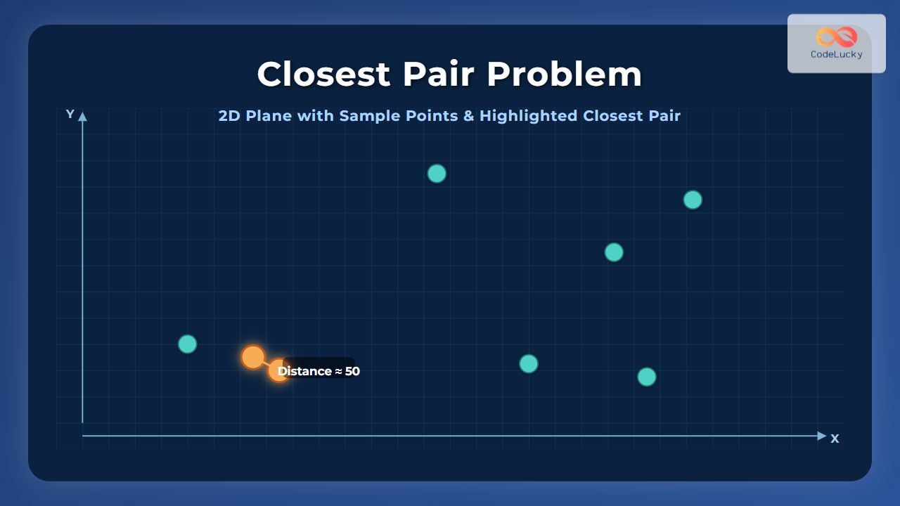
The Closest Pair Problem is a fundamental computational geometry challenge that involves finding the two points closest to each other in a set of points on a plane. This problem is critical in many domains such as computer graphics, geographic information systems (GIS), clustering analysis, and more. Naively, checking every pair of points takes O(n²) time, but efficient algorithms can solve it in O(n log n) time using divide and conquer techniques.
Understanding the Closest Pair Problem
Given n points in a 2D plane, the goal is to identify the pair with the minimal Euclidean distance between them. Formally, if the points are represented as P = {p₁, p₂, ..., pₙ}, find (pᵢ, pⱼ) such that the distance d(pᵢ, pⱼ) is minimized.
Applications
- Collision detection in simulations and games
- Clustering algorithms for pattern recognition
- Network design and routing optimization
- Geospatial data analysis
Naive Approach: Brute Force
The brute-force method checks every possible pair of points and calculates the distance between them:
- Number of pairs =
n(n-1)/2 - Time complexity =
O(n²)
This is straightforward but inefficient for large data sets.
Efficient Solution: Divide and Conquer Algorithm
The key breakthrough is to use a divide and conquer strategy similar to merge sort to achieve O(n log n) time complexity. The general outline is:
- Sort the points by their x-coordinates.
- Recursively divide points into two halves.
- Find the closest pair in the left half and the right half.
- Find the closest pair that crosses the division line.
- Return the minimum of these distances.
How the Crossing Pair Check Works
After finding the smallest distances δ from both halves, only points within δ distance of the dividing line are considered for cross-boundary pairs. This drastically reduces the number of comparisons.
Step-by-step Algorithm Example
Consider the points set:
P = {(2, 3), (12, 30), (40, 50), (5, 1), (12, 10), (3, 4)}Step 1: Sort points by x:
(2, 3), (3, 4), (5, 1), (12, 10), (12, 30), (40, 50)Step 2: Recursively divide:
- Left:
(2,3), (3,4), (5,1) - Right:
(12,10), (12,30), (40,50)
Step 3: Recursively find closest pairs in each half.
For Left:
– Distances:
– (2,3)-(3,4) = √2 ≈ 1.41
– (2,3)-(5,1) = √13 ≈ 3.6
– (3,4)-(5,1) = √13 ≈ 3.6
– Closest pair: (2,3) & (3,4) at 1.41
For Right:
– Distances:
– (12,10)-(12,30) = 20
– (12,10)-(40,50) = ~50.38
– (12,30)-(40,50) = ~36.06
– Closest pair: (12,10) & (12,30) at 20
Step 4: Check across midpoint (x=5 to 12). Points near midline within distance 1.41 (minimum found) are filtered and compared by y-coordinate.
Result: The closest pair is (2,3) and (3,4) with distance ~1.41
Python Implementation
def closest_pair(points):
    def dist(a, b):
        return ((a[0]-b[0])**2 + (a[1]-b[1])**2)**0.5

    def closest_split_pair(px, py, delta, best_pair):
        mid_x = px[len(px)//2][0]
        sy = [p for p in py if mid_x - delta <= p[0] <= mid_x + delta]
        best = delta
        ln = len(sy)
        for i in range(ln):
            for j in range(i+1, min(i+7, ln)):
                p, q = sy[i], sy[j]
                dst = dist(p, q)
                if dst < best:
                    best = dst
                    best_pair = (p, q)
        return best, best_pair

    def recursive(px, py):
        if len(px) <= 3:
            min_d = float('inf')
            pair = None
            for i in range(len(px)):
                for j in range(i+1, len(px)):
                    d = dist(px[i], px[j])
                    if d < min_d:
                        min_d = d
                        pair = (px[i], px[j])
            return min_d, pair

        mid = len(px)//2
        Qx = px[:mid]
        Rx = px[mid:]
        midpoint = px[mid][0]
        Qy = list(filter(lambda p: p[0] <= midpoint, py))
        Ry = list(filter(lambda p: p[0] > midpoint, py))

        (dl, pair_left) = recursive(Qx, Qy)
        (dr, pair_right) = recursive(Rx, Ry)

        delta = min(dl, dr)
        best_pair = pair_left if dl < dr else pair_right

        (ds, pair_split) = closest_split_pair(px, py, delta, best_pair)

        if delta < ds:
            return delta, best_pair
        else:
            return ds, pair_split

    px = sorted(points, key=lambda p: p[0])
    py = sorted(points, key=lambda p: p[1])
    distance, pair = recursive(px, py)
    return distance, pair

# Example usage
points = [(2,3), (12,30), (40,50), (5,1), (12,10), (3,4)]
dist, closest = closest_pair(points)
print("Closest distance:", dist)
print("Closest points:", closest)
Visualizing the Closest Pair Problem
Visual tools help in understanding point divisions and the narrowing of candidate points in the δ-strip near the divide line.
Performance and Complexity
The divide and conquer closest pair algorithm runs in O(n log n) time due to:
- Initial sorting in
O(n log n) - Recursive division leads to
2T(n/2) - Merge step and cross-pair check in
O(n)
This efficiency enables handling large spatial data with speed while preserving correctness.
Summary & Best Practices
- The brute force approach is simple but quadratic and unsuitable for large inputs.
- Divide and conquer with plane sorting and δ-strip filtering offers optimal performance.
- Sorting points by both x and y coordinates is essential for efficiency.
- Implementation details like limiting cross comparisons to 7 neighbors in the strip are crucial.
For practical uses, consider pre-processing with spatial data structures like KD-Trees for dynamic nearest-neighbor queries, but for static datasets, the divide and conquer method remains the gold standard.


