Memory allocation is a fundamental aspect of operating system design that determines how programs and data are stored and accessed in computer memory. Understanding the different allocation techniques is crucial for system administrators, developers, and anyone working with system-level programming.
What is Memory Allocation?
Memory allocation refers to the process of assigning portions of physical memory (RAM) to running processes and programs. The operating system’s memory manager is responsible for tracking which memory locations are free, which are occupied, and efficiently distributing available memory among competing processes.
The choice of memory allocation technique directly impacts system performance, memory utilization efficiency, and the complexity of memory management operations. Modern operating systems employ sophisticated algorithms to balance these factors while ensuring system stability and optimal resource usage.
Types of Memory Allocation Techniques
Memory allocation techniques are broadly categorized into two main approaches:
- Contiguous Memory Allocation – Allocates consecutive memory blocks
- Non-contiguous Memory Allocation – Allows scattered memory block allocation
Contiguous Memory Allocation
Contiguous memory allocation assigns consecutive memory addresses to a process. This means all memory locations allocated to a program are adjacent to each other in physical memory, creating a single continuous block.
Characteristics of Contiguous Allocation
- Simple memory management with minimal overhead
- Fast access due to locality of reference
- Easy implementation of memory protection
- Direct mapping between logical and physical addresses
- Susceptible to external fragmentation

Types of Contiguous Allocation Strategies
1. Fixed Partitioning
Memory is divided into fixed-size partitions at system startup. Each process is allocated to a partition that can accommodate its size requirements.
Memory Layout Example:
┌─────────────────┐ 0KB
│   OS Kernel     │
├─────────────────┤ 100KB
│   Partition 1   │ (200KB)
├─────────────────┤ 300KB
│   Partition 2   │ (200KB)
├─────────────────┤ 500KB
│   Partition 3   │ (300KB)
├─────────────────┤ 800KB
│   Partition 4   │ (200KB)
└─────────────────┘ 1000KB
Advantages:
- Simple implementation and management
- Fast allocation and deallocation
- No external fragmentation
Disadvantages:
- Internal fragmentation when process size < partition size
- Limited number of concurrent processes
- Poor memory utilization
2. Dynamic Partitioning
Partitions are created dynamically based on process requirements. The system allocates exactly the amount of memory requested by each process.
Initial State:
┌─────────────────┐ 0KB
│   OS Kernel     │
├─────────────────┤ 100KB
│                 │
│   Free Memory   │
│                 │
└─────────────────┘ 1000KB

After Process Allocation:
┌─────────────────┐ 0KB
│   OS Kernel     │
├─────────────────┤ 100KB
│   Process A     │ (150KB)
├─────────────────┤ 250KB
│   Process B     │ (200KB)
├─────────────────┤ 450KB
│   Free Memory   │
└─────────────────┘ 1000KB
Allocation Algorithms for Dynamic Partitioning
First Fit Algorithm
Allocates the first available free block that is large enough to accommodate the process.
def first_fit(memory_blocks, process_size):
    for i, block in enumerate(memory_blocks):
        if block['free'] and block['size'] >= process_size:
            # Allocate memory
            block['free'] = False
            block['process'] = current_process
            return block['start_address']
    return None  # No suitable block found
Best Fit Algorithm
Searches for the smallest free block that can accommodate the process, minimizing wasted space.
def best_fit(memory_blocks, process_size):
    best_block = None
    min_waste = float('inf')

    for block in memory_blocks:
        if block['free'] and block['size'] >= process_size:
            waste = block['size'] - process_size
            if waste < min_waste:
                min_waste = waste
                best_block = block

    if best_block:
        best_block['free'] = False
        best_block['process'] = current_process
        return best_block['start_address']
    return None
Worst Fit Algorithm
Allocates the largest available free block, leaving the maximum remaining free space.
Memory Compaction
To address external fragmentation in dynamic partitioning, operating systems use memory compaction – relocating allocated partitions to create larger contiguous free spaces.

Non-contiguous Memory Allocation
Non-contiguous memory allocation allows a process to occupy multiple non-adjacent memory blocks. This approach eliminates the requirement for consecutive memory addresses, providing greater flexibility in memory management.
Advantages of Non-contiguous Allocation
- Eliminates external fragmentation
- Better memory utilization
- Supports virtual memory implementation
- Allows processes larger than available contiguous memory
- Facilitates memory sharing between processes
Disadvantages of Non-contiguous Allocation
- Complex memory management overhead
- Address translation complexity
- Potential for internal fragmentation
- Hardware support requirements
Paging – A Non-contiguous Technique
Paging divides physical memory into fixed-size blocks called frames and logical memory into blocks of the same size called pages. The operating system maintains a page table to map logical pages to physical frames.
Paging Implementation

Page Table Structure
Page Table Example (4KB pages):
┌─────────────┬─────────────┬─────────────┐
│ Page Number │ Frame Number│ Valid Bit   │
├─────────────┼─────────────┼─────────────┤
│      0      │      5      │      1      │
│      1      │      2      │      1      │
│      2      │      8      │      1      │
│      3      │      1      │      1      │
│      4      │      -      │      0      │
└─────────────┴─────────────┴─────────────┘
Address Translation in Paging
The memory management unit (MMU) translates logical addresses to physical addresses using the following process:
- Extract page number from the logical address
- Look up frame number in the page table
- Combine frame number with page offset to form physical address
Address Translation Example:
Logical Address: 8196 (binary: 10000000000100)
Page Size: 4KB (4096 bytes)

Page Number = 8196 / 4096 = 2
Page Offset = 8196 % 4096 = 4

From Page Table: Page 2 → Frame 8
Physical Address = (Frame 8 × 4096) + 4 = 32772
Multi-level Paging
For systems with large address spaces, single-level page tables become impractically large. Multi-level paging breaks the page table into smaller, manageable pieces.

Segmentation – Another Non-contiguous Approach
Segmentation divides programs into logical segments such as code, data, and stack. Each segment can vary in size and is allocated non-contiguously in memory.
Segment Table Structure
Segment Table:
┌─────────────┬─────────────┬─────────────┬─────────────┐
│ Segment #   │ Base Address│ Limit       │ Permissions │
├─────────────┼─────────────┼─────────────┼─────────────┤
│      0      │    1000     │     500     │    R-X      │ Code
│      1      │    2000     │     300     │    RW-      │ Data
│      2      │    3500     │     200     │    RW-      │ Stack
│      3      │    4000     │     150     │    R--      │ Constants
└─────────────┴─────────────┴─────────────┴─────────────┘
Segmented Paging
Many modern systems combine segmentation and paging to leverage benefits of both techniques. Each segment is divided into pages, providing both logical organization and efficient memory utilization.

Comparison: Contiguous vs Non-contiguous Allocation
| Aspect | Contiguous Allocation | Non-contiguous Allocation |
|---|---|---|
| Memory Utilization | Lower due to fragmentation | Higher, better space efficiency |
| Implementation Complexity | Simple and straightforward | Complex with hardware support |
| Address Translation | Direct, minimal overhead | Requires translation tables |
| External Fragmentation | Significant problem | Eliminated completely |
| Internal Fragmentation | Possible in fixed partitioning | Minimal in paging systems |
| Memory Protection | Simple base-limit registers | Page-level protection bits |
| Virtual Memory Support | Limited or impossible | Full virtual memory support |
| Process Size Limitations | Limited by largest free block | Can exceed physical memory |
Performance Considerations
Memory Access Patterns
The choice between contiguous and non-contiguous allocation significantly impacts system performance based on memory access patterns:
- Sequential Access: Contiguous allocation provides better cache performance
- Random Access: Non-contiguous allocation offers more flexibility
- Large Data Sets: Non-contiguous allocation prevents memory starvation
Translation Lookaside Buffer (TLB)
In non-contiguous systems, the TLB caches recent address translations to reduce the overhead of page table lookups:
TLB Hit Rate Impact:
- TLB Hit: ~1 cycle access time
- TLB Miss: ~100+ cycles (page table walk)
- Effective Access Time = Hit Rate × Hit Time + Miss Rate × Miss Time
Modern Memory Management Trends
Hybrid Approaches
Contemporary operating systems often employ hybrid strategies combining multiple allocation techniques:
- Kernel Space: Often uses contiguous allocation for critical data structures
- User Space: Primarily uses paging for process memory
- Device Drivers: May require contiguous memory for DMA operations
- File Systems: Use both approaches depending on file size and access patterns
Large Page Support
Modern processors support multiple page sizes (4KB, 2MB, 1GB) to reduce TLB pressure for large applications while maintaining granular control for smaller allocations.
Implementation Examples
Simple Memory Allocator
class MemoryAllocator:
    def __init__(self, total_memory):
        self.memory_blocks = [
            {'start': 0, 'size': total_memory, 'free': True, 'process': None}
        ]

    def allocate(self, process_id, size, algorithm='first_fit'):
        if algorithm == 'first_fit':
            return self._first_fit(process_id, size)
        elif algorithm == 'best_fit':
            return self._best_fit(process_id, size)
        return None

    def deallocate(self, process_id):
        for block in self.memory_blocks:
            if block['process'] == process_id:
                block['free'] = True
                block['process'] = None
        self._coalesce()  # Merge adjacent free blocks

    def _first_fit(self, process_id, size):
        for i, block in enumerate(self.memory_blocks):
            if block['free'] and block['size'] >= size:
                self._split_block(i, size, process_id)
                return block['start']
        return None
Page Table Implementation
class PageTable:
    def __init__(self, page_size=4096):
        self.page_size = page_size
        self.entries = {}  # page_number -> frame_number

    def map_page(self, page_number, frame_number):
        self.entries[page_number] = {
            'frame': frame_number,
            'valid': True,
            'dirty': False,
            'referenced': False
        }

    def translate_address(self, logical_address):
        page_number = logical_address // self.page_size
        page_offset = logical_address % self.page_size

        if page_number not in self.entries or not self.entries[page_number]['valid']:
            raise PageFaultException(f"Page {page_number} not in memory")

        frame_number = self.entries[page_number]['frame']
        physical_address = (frame_number * self.page_size) + page_offset

        # Update reference bit for LRU replacement
        self.entries[page_number]['referenced'] = True

        return physical_address
Best Practices and Recommendations
When to Use Contiguous Allocation
- Real-time systems requiring predictable memory access
- Embedded systems with limited hardware capabilities
- Device driver development for DMA operations
- High-performance computing applications with sequential access patterns
When to Use Non-contiguous Allocation
- General-purpose operating systems
- Multi-user environments with varying process sizes
- Systems requiring virtual memory support
- Applications with unpredictable memory access patterns
Optimization Strategies
- Memory Pool Allocation: Pre-allocate fixed-size blocks for frequent allocations
- Buddy System: Combine benefits of both approaches for efficient allocation
- NUMA Awareness: Consider processor-memory topology in allocation decisions
- Huge Page Usage: Leverage large pages for memory-intensive applications
Understanding memory allocation techniques is essential for developing efficient systems and applications. While contiguous allocation offers simplicity and performance benefits in specific scenarios, non-contiguous allocation provides the flexibility and efficiency required by modern computing environments. The choice between these approaches depends on specific system requirements, hardware constraints, and performance objectives.
As computing systems continue evolving, hybrid approaches that intelligently combine multiple allocation strategies are becoming increasingly prevalent, offering the benefits of both contiguous and non-contiguous techniques while minimizing their respective drawbacks.
Related Posts
Memory Management in Operating System: Virtual and Physical Memory Fundamentals
Introduction to Memory Management Memory management is one of the most critical functions of an operating system, responsible for efficiently...

C Memory Management: Advanced Techniques and Best Practices
Memory management is a critical aspect of C programming that can make or break your application's performance and reliability. In...
Segmentation in OS: Memory Management Through Logical Address Space Division
Introduction to Segmentation in Operating Systems Segmentation is a fundamental memory management technique in operating systems that divides the logical...
Windows Memory Management: Virtual Memory Implementation and Optimization Guide
Introduction to Windows Virtual Memory Windows virtual memory is a sophisticated memory management system that allows programs to use more...
File Allocation Methods: Contiguous, Linked and Indexed Storage Techniques
Understanding File Allocation Methods in Operating Systems File allocation methods are fundamental techniques used by operating systems to organize and...
Virtual Memory in OS: Complete Guide to Paging, Segmentation and Address Translation
Virtual memory is one of the most fundamental concepts in modern operating systems, enabling efficient memory management and providing crucial...
Dynamic Memory Allocation: malloc, calloc and free Functions in C Programming
What is Dynamic Memory Allocation? Dynamic memory allocation is a fundamental concept in operating systems and programming that allows programs...
Garbage Collection in Operating System: Complete Guide to Automatic Memory Management
What is Garbage Collection in Operating Systems? Garbage collection is an automatic memory management technique used by operating systems and...

C Memory Management: Dynamic Allocation with malloc() and free()
Memory management is a crucial aspect of C programming that every developer must master. In this comprehensive guide, we'll dive...
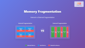
Memory Fragmentation: Internal vs External Fragmentation in Operating Systems
Memory fragmentation is one of the most critical challenges in operating system memory management, directly impacting system performance and resource...
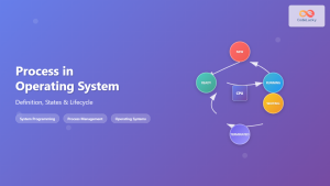
Process in Operating System: Complete Guide to Definition, States and Lifecycle
What is a Process in Operating System? A process is a program in execution that consists of the program code...
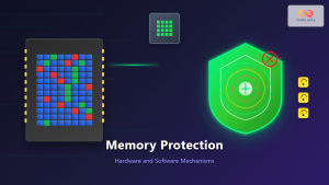
Memory Protection: Hardware and Software Mechanisms for Secure Computing
Understanding Memory Protection in Modern Computing Memory protection is a fundamental security mechanism that prevents programs from accessing memory regions...
- What is Memory Allocation?
- Types of Memory Allocation Techniques
- Contiguous Memory Allocation
- Non-contiguous Memory Allocation
- Paging – A Non-contiguous Technique
- Segmentation – Another Non-contiguous Approach
- Comparison: Contiguous vs Non-contiguous Allocation
- Performance Considerations
- Modern Memory Management Trends
- Implementation Examples
- Best Practices and Recommendations