Excel structured references revolutionize how you work with tables by replacing traditional cell references with intuitive, readable formula syntax. Instead of cryptic references like A2:C10, you can use meaningful names like Sales[Amount] that automatically adjust as your table grows or shrinks.
What Are Excel Structured References?
Structured references are a special syntax used in Excel tables that make formulas more readable and maintainable. When you convert a range to a table using Insert > Table or Ctrl+T, Excel automatically enables structured references for that data.
The key advantages include:
- Readability: Formula purposes become immediately clear
- Automatic expansion: References adjust when adding rows or columns
- Error reduction: Less prone to incorrect cell references
- Maintenance: Easier to update and debug formulas
Basic Structured Reference Syntax
The fundamental structure follows this pattern:
TableName[ColumnName]
For example, if you have a table named “SalesData” with a column “Revenue”, the structured reference would be:
=SalesData[Revenue]Table Name Rules
Excel automatically assigns table names like “Table1”, “Table2”, but you should rename them for clarity:
- Names must start with a letter or underscore
- Cannot contain spaces (use underscores instead)
- Cannot match cell references (avoid names like “A1” or “R1C1”)
- Maximum 255 characters
To rename a table, select any cell within it and use the Table Name box in the Table Design tab.
Column Reference Syntax
Single Column References
Reference an entire column using brackets:
=SUM(SalesData[Amount])
=AVERAGE(Products[Price])
=MAX(Inventory[Quantity])
Multiple Column References
Select multiple columns using the range operator:
=SUM(SalesData[Jan]:[Dec])
=AVERAGE(Budget[Q1]:[Q4])
Column Headers with Spaces
When column headers contain spaces or special characters, Excel handles them automatically:
=SUM(SalesData[Net Sales])
=AVERAGE(Employees[Years of Service])
Row-Specific References
This Row (@) Reference
The @ symbol references the current row, particularly useful in calculated columns:
=[@Price] * [@Quantity]
=IF([@Status]="Active", [@Amount], 0)
Excel often adds the @ automatically when you create formulas within table rows.
Specific Row References
While less common, you can reference specific rows:
=SalesData[@[Amount]:[Tax]]  // Current row, multiple columns
=SalesData[#Headers]         // Header row only
=SalesData[#Data]           // Data rows only
=SalesData[#Totals]         // Total row only
Special Table Areas
Table Sections
Excel provides special identifiers for different table sections:
| Reference | Description | Example |
|---|---|---|
[#All] |
Entire table including headers | SalesData[#All] |
[#Data] |
Data rows only | SalesData[#Data] |
[#Headers] |
Header row only | SalesData[#Headers] |
[#Totals] |
Total row only | SalesData[#Totals] |
[#This Row] |
Current row | SalesData[#This Row] |
Combining Sections with Columns
=SUM(SalesData[Amount][#Data])        // Sum data rows only
=COUNTA(Products[Name][#Headers])     // Count header cells
=AVERAGE(Scores[Math][#Data])         // Average excluding headers
Advanced Structured Reference Techniques
Intersections and Ranges
Create complex references using intersections:
=SUM(SalesData[Jan]:[Mar])                    // Q1 columns
=AVERAGE(SalesData[@Jan]:[@Mar])              // Current row Q1
=SUM(SalesData[Amount] SalesData[#Data])      // Intersection syntax
External Table References
Reference tables in other worksheets:
=SUM(Sheet2!SalesData[Amount])
=VLOOKUP(A2, OtherSheet!Products[#All], 2, FALSE)
Using with Array Formulas
Structured references work seamlessly with array formulas:
=SUM(IF(SalesData[Region]="North", SalesData[Amount], 0))
=SUMPRODUCT((Products[Category]="Electronics") * Products[Sales])
Common Functions with Structured References
Statistical Functions
=AVERAGE(SalesData[Revenue])
=STDEV(Products[Price])
=MEDIAN(Scores[Mathematics])
=PERCENTILE(SalesData[Amount], 0.9)
Lookup Functions
=VLOOKUP(E2, Products[#All], 3, FALSE)
=INDEX(SalesData[Name], MATCH(MAX(SalesData[Amount]), SalesData[Amount], 0))
=XLOOKUP(F2, Employees[ID], Employees[Salary])
Conditional Functions
=SUMIF(SalesData[Region], "West", SalesData[Amount])
=COUNTIFS(Products[Category], "Electronics", Products[Stock], ">100")
=AVERAGEIF(Scores[Subject], "Math", Scores[Grade])
Best Practices for Structured References
Naming Conventions
- Use descriptive table names: “SalesData” instead of “Table1”
- Keep column headers clear: “Unit_Price” instead of “UP”
- Avoid abbreviations: “Quantity” instead of “Qty”
- Use consistent formatting: CamelCase or snake_case throughout
Formula Organization
- Group related calculations: Keep similar formulas together
- Document complex formulas: Add comments explaining logic
- Test edge cases: Verify formulas work with empty tables
- Use meaningful intermediate calculations: Break complex formulas into steps
Troubleshooting Common Issues
Reference Errors
Problem: #REF! errors when referencing renamed columns
Solution: Excel usually updates automatically, but manually refresh with Ctrl+Alt+F9
Circular References
Problem: Formulas referencing themselves
Solution: Check calculated columns aren’t referencing their own column
Performance Issues
Problem: Slow calculation with large tables
Solution: Use specific references like [#Data] instead of [#All]
Converting Between Reference Types
Traditional to Structured
When you convert a range to a table, Excel doesn’t automatically update existing formulas. Update them manually:
Before: =SUM(A2:A100)
After:  =SUM(SalesData[Amount])
Structured to Traditional
Use Formulas > Name Manager to see how Excel interprets structured references as traditional ranges.
Performance Optimization Tips
- Limit table size: Keep tables under 100,000 rows for optimal performance
- Use specific sections: Reference
[#Data]instead of entire columns - Minimize volatile functions: Combine structured references with INDIRECT sparingly
- Consider calculation mode: Switch to manual calculation for large datasets
Advanced Examples and Use Cases
Dynamic Dashboard Creation
=SUMIFS(SalesData[Amount], SalesData[Date], ">="&DATE(YEAR(TODAY()),1,1),
        SalesData[Region], Dashboard[Selected_Region])
Conditional Formatting with Structured References
Create rules that automatically apply to new table rows:
=Products[@Stock]Data Validation Lists
Use table columns for dynamic dropdown lists:
=Products[Category]Excel structured references transform complex spreadsheet formulas into readable, maintainable code. By mastering this syntax, you'll create more robust, professional spreadsheets that adapt automatically as your data grows. Remember to use descriptive names, test your formulas thoroughly, and leverage Excel's automatic expansion features to build truly dynamic worksheets.
Related Posts

Excel TABLE Function: Complete Guide to Structured Data Management and Advanced Formulas
What is the Excel TABLE Function? The Excel TABLE function is a powerful feature that converts regular cell ranges into...
Excel COLUMN Function: Complete Guide to Column Number References
The Excel COLUMN function is a fundamental lookup and reference function that returns the column number of a specified cell...
Excel ROW Function: Complete Guide to Row Number Formula and Syntax
The Excel ROW function is one of the most fundamental yet powerful functions in Microsoft Excel, designed to return the...

Excel OFFSET Function: Dynamic Reference Formula for Advanced Data Management
The Excel OFFSET function is one of the most powerful yet underutilized tools for creating dynamic references in spreadsheets. This...
Excel CELL Function: Complete Guide to Cell Information Formula Syntax
The CELL function in Microsoft Excel is a powerful information function that returns specific details about the formatting, location, or...
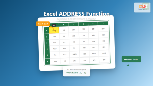
Excel ADDRESS Function: Complete Guide to Dynamic Cell Reference Creation
The Excel ADDRESS function is a powerful text function that creates cell references as text strings based on row and...

Excel INDIRECT Function: Complete Guide to Dynamic Cell Reference Creation
The INDIRECT function in Microsoft Excel is a powerful reference function that allows you to create dynamic cell references from...
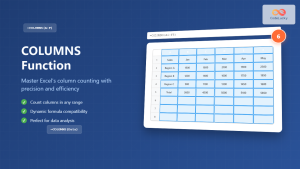
Excel COLUMNS Function: Master Column Counting with Practical Examples
The Excel COLUMNS function is a powerful built-in tool that counts the number of columns in a specified range or...

Excel ROWS Function: Complete Guide to Count Rows with Formula Syntax Examples
What is the Excel ROWS Function? The ROWS function in Microsoft Excel is a built-in lookup and reference function that...
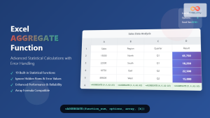
Excel AGGREGATE Function: Complete Guide to Advanced Statistical Calculations
Excel's AGGREGATE function is one of the most powerful and versatile statistical functions available in Microsoft Excel. Unlike traditional statistical...

Excel TYPE Function: Complete Guide to Data Type Detection and Validation
The Excel TYPE function is a powerful information function that identifies the data type of a value in a cell...
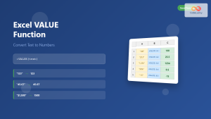
Excel VALUE Function: Complete Guide to Text-to-Number Conversion
The Excel VALUE function is a powerful data conversion tool that transforms text strings containing numeric values into actual numbers...