Searching is one of the most fundamental operations in computer science. Whether it’s finding a number in an array, looking up a word in a dictionary, or querying a database, search algorithms play a vital role. Choosing the right search algorithm can drastically improve efficiency depending on the dataset type, structure, and access requirements. This article provides a detailed comparison of search algorithms, complete with examples, complexity analysis, and visual diagrams to help you decide which algorithm to use when.
Why Search Algorithms Matter
Search efficiency directly impacts software performance. A naive search might suffice for small datasets, while large-scale applications require optimized algorithms tailored to the data structure. For example, search in an unsorted dataset differs significantly from search in a sorted one.
Popular Search Algorithms
Let’s compare the most common search algorithms and analyze their performance characteristics.
1. Linear Search
Linear Search (or Sequential Search) is the simplest technique. It checks elements one by one until the target is found or the list ends.
def linear_search(arr, target):
    for i, value in enumerate(arr):
        if value == target:
            return i
    return -1

print(linear_search([10, 20, 30, 40, 50], 30))  # Output: 2
Complexity:
- Time Complexity: O(n)
- Best Case: O(1) (target at first position)
- Worst Case: O(n)
- Space Complexity: O(1)
When to Use: Use Linear Search for small datasets or unsorted data. It requires no pre-processing.
2. Binary Search
Binary Search is a highly efficient method but requires the dataset to be sorted. It repeatedly divides the search range in half.
def binary_search(arr, target):
    left, right = 0, len(arr) - 1
    while left <= right:
        mid = (left + right) // 2
        if arr[mid] == target:
            return mid
        elif arr[mid] < target:
            left = mid + 1
        else:
            right = mid - 1
    return -1

print(binary_search([10, 20, 30, 40, 50], 40))  # Output: 3
Complexity:
- Time Complexity: O(log n)
- Space Complexity: O(1) for iterative implementation
When to Use: Ideal when the dataset is large and already sorted. Very efficient compared to Linear Search.
3. Ternary Search
Ternary Search divides the array into three parts instead of two. It’s similar to Binary Search but checks two mid-points at each step.
def ternary_search(arr, target, left, right):
    if left > right:
        return -1
    mid1 = left + (right - left) // 3
    mid2 = right - (right - left) // 3
    if arr[mid1] == target:
        return mid1
    if arr[mid2] == target:
        return mid2
    if target < arr[mid1]:
        return ternary_search(arr, target, left, mid1-1)
    elif target > arr[mid2]:
        return ternary_search(arr, target, mid2+1, right)
    else:
        return ternary_search(arr, target, mid1+1, mid2-1)

arr = [10, 20, 30, 40, 50, 60, 70]
print(ternary_search(arr, 60, 0, len(arr)-1))  # Output: 5
Complexity: O(log3 n), very close to Binary Search in practice.
When to Use: Prefer Binary Search usually, as dividing the range into three doesn’t bring significant benefits and adds computation overhead.
4. Jump Search
Jump Search works on sorted arrays. It checks elements at fixed intervals (jumps) and then performs Linear Search in the identified block.
import math

def jump_search(arr, target):
    n = len(arr)
    step = int(math.sqrt(n))
    prev = 0
    while arr[min(step, n)-1] < target:
        prev = step
        step += int(math.sqrt(n))
        if prev >= n:
            return -1
    for i in range(prev, min(step, n)):
        if arr[i] == target:
            return i
    return -1

print(jump_search([10, 20, 30, 40, 50, 60], 50))  # Output: 4
Complexity: O(√n)
When to Use: Useful where random access is allowed (like arrays) and data is sorted.
5. Interpolation Search
Interpolation Search improves on Binary Search when data is uniformly distributed. It estimates the probable position of the target and checks accordingly.
def interpolation_search(arr, target):
    low, high = 0, len(arr) - 1
    while low <= high and arr[low] <= target <= arr[high]:
        pos = low + ((target - arr[low]) * (high - low) //
                    (arr[high] - arr[low]))
        if arr[pos] == target:
            return pos
        elif arr[pos] < target:
            low = pos + 1
        else:
            high = pos - 1
    return -1

arr = [10, 20, 30, 40, 50, 60, 70]
print(interpolation_search(arr, 40))  # Output: 3
Complexity:
- Best Case: O(1)
- Average Case: O(log log n)
- Worst Case: O(n) (when distribution is skewed)
When to Use: Best for uniformly distributed sorted data like searching for student IDs or values in numerical ranges.
Comparison Table of Search Algorithms
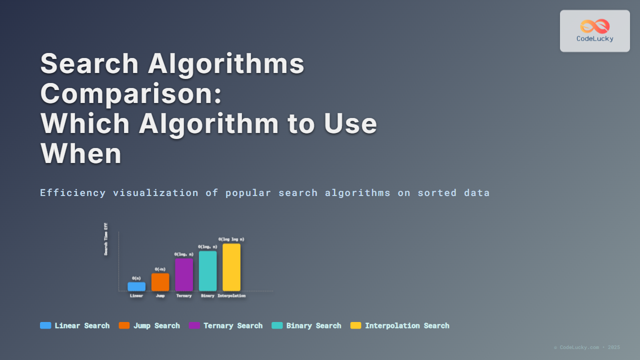
| Algorithm | Best Case | Average Case | Worst Case | Sorted Data Required? |
|---|---|---|---|---|
| Linear Search | O(1) | O(n) | O(n) | No |
| Binary Search | O(1) | O(log n) | O(log n) | Yes |
| Ternary Search | O(1) | O(log n) | O(log n) | Yes |
| Jump Search | O(√n) | O(√n) | O(n) | Yes |
| Interpolation Search | O(1) | O(log log n) | O(n) | Yes |
Which Algorithm to Use When?
- Small or unsorted dataset: Use Linear Search.
- Large sorted dataset: Use Binary Search (preferred) or Ternary Search.
- Sorted dataset with random access: Use Jump Search as a middle ground.
- Uniformly distributed sorted data: Interpolation Search gives best results.
Conclusion
The choice of search algorithm depends heavily on the dataset’s properties and performance requirements. For most practical cases, Binary Search is the go-to method for sorted data, while Linear Search is sufficient for small or unsorted datasets. Advanced algorithms like Interpolation Search shine only under specific conditions of data distribution. Understanding these subtle differences helps you build more efficient software systems.
Now that you’ve understood search algorithms comparison, you can carefully pick the right one based on your application’s requirements and data nature.

