Neural networks form the backbone of modern deep learning models, enabling machines to learn from data and perform complex tasks like image recognition, natural language processing, and more. The fundamental algorithm that empowers these networks to improve their accuracy is backpropagation. This article explores how neural network backpropagation works, the mathematics behind it, and the practical steps to train deep learning models effectively—accompanied by visual explanations for clarity.
Understanding Neural Network Backpropagation
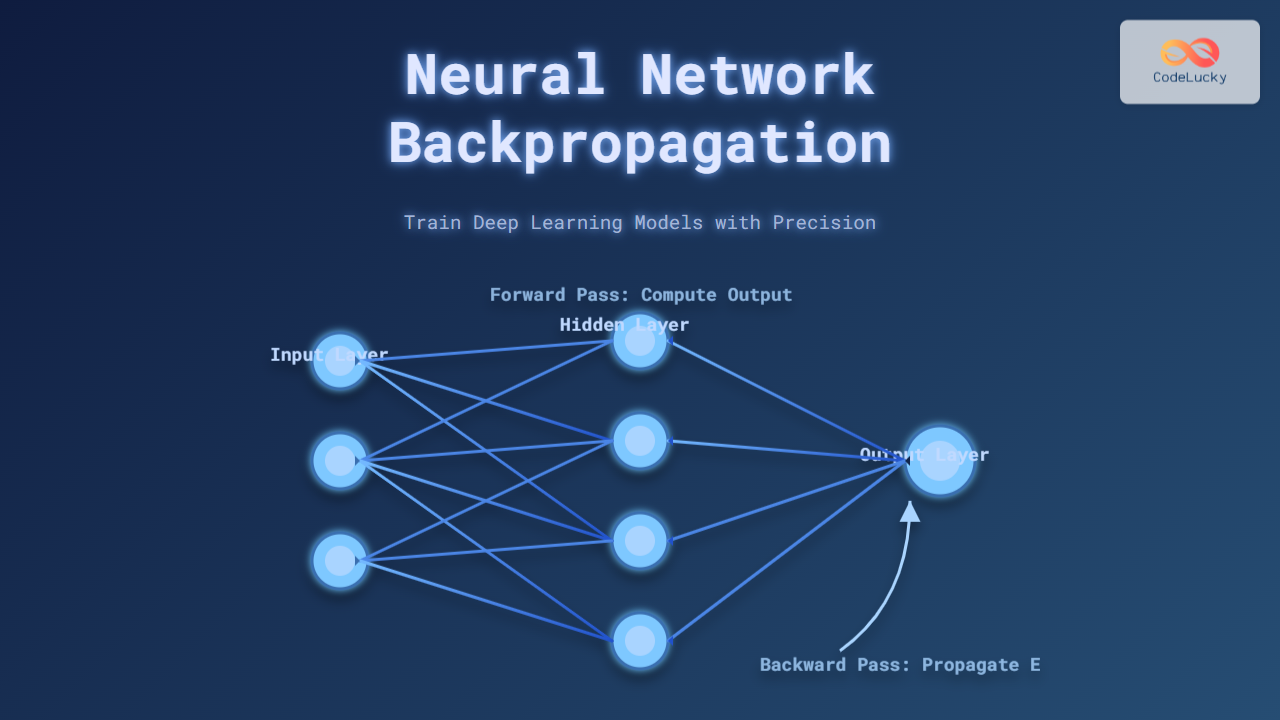
Backpropagation is a supervised learning technique used for updating the weights of a neural network. The core objective is to minimize the difference between the predicted output and the actual target, called the loss. This process propagates the error backward from the output to the input layers, adjusting weights at each layer to reduce future errors.
Why Backpropagation Is Essential
- Efficient Learning: It allows deep networks to learn complex patterns by optimizing weight parameters.
- Error Minimization: It systematically reduces prediction errors using gradient descent.
- Scalability: Works for networks of any size, including deep architectures with many layers.
The Math Behind Backpropagation
At the heart of backpropagation is the chain rule from calculus, which breaks down the derivative of the loss function with respect to each weight into manageable parts.
Key Components:
- Forward Pass: Compute the output of the network for given inputs.
- Loss Function: Measure how far the prediction is from the target (e.g., mean squared error, cross-entropy).
- Backward Pass: Compute gradients of loss with respect to weights using derivatives.
- Weight Update: Adjust weights by moving in the direction opposite the gradient (Gradient Descent).
Mathematically for a single weight \( w \):
\[
w = w - \eta \times \frac{\partial L}{\partial w}
\]
Where \( \eta \) is the learning rate controlling the step size.
Step-by-Step Backpropagation Example
Consider a simple neural network with one input layer, one hidden layer, and one output layer. Let’s walk through backpropagation training on a single data point.
- Forward Pass:
- Input: \( x = 0.5 \)
- Weights: \( w_1 = 0.4 \), \( w_2 = 0.6 \)
- Hidden Layer Activation: \( h = \sigma(w_1 \times x) \)
- Output: \( y_{pred} = \sigma(w_2 \times h) \)
- True Output: \( y = 1 \)
- Calculate Loss: Mean Squared Error \( L = \frac{1}{2}(y – y_{pred})^2 \)
- Backward Pass: Compute gradients \( \frac{\partial L}{\partial w_2} \), \( \frac{\partial L}{\partial w_1} \) using chain rule.
- Update Weights: Apply gradient descent update formula with learning rate \( \eta \).
This iterative approach allows the model to tune weights gradually.
Interactive Neural Network Backpropagation Diagram
Practical Tips to Train Neural Networks Using Backpropagation
- Normalize Inputs: Helps faster convergence by scaling feature values.
- Choose Suitable Activation Functions: ReLU for hidden layers and sigmoid/softmax for outputs.
- Adjust Learning Rate: Too large causes instability; too small slows training.
- Regularize Models: Techniques like dropout prevent overfitting.
- Use Batch Gradient Descent: Process multiple samples to stabilize updates.
Backpropagation Algorithm Pseudocode
Initialize weights randomly

For each epoch:
  For each training example (x, y):
    1. Forward Pass: Calculate predicted output y_pred
    2. Compute Loss: L(y, y_pred)
    3. Backward Pass: Calculate gradients ∂L/∂w using chain rule
    4. Update Weights: w = w - η * ∂L/∂w

Repeat until convergence or max epochs reached
Conclusion
Backpropagation remains the fundamental algorithm to efficiently train deep neural networks by iteratively minimizing prediction errors via gradient descent. Understanding its mechanism is vital for developing and tuning high-performing AI models. This detailed guide with visual explanations equips machine learning practitioners with the knowledge to implement backpropagation from scratch and optimize deep learning workflows.


