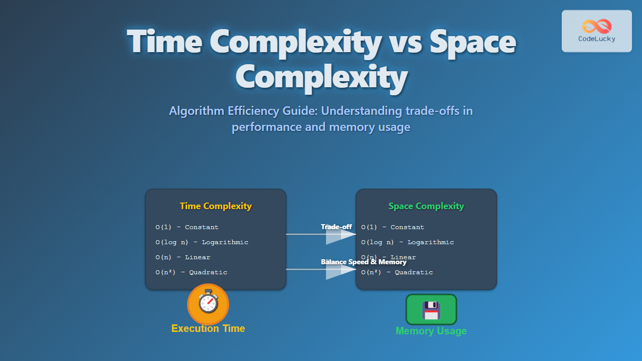
Time Complexity vs Space Complexity: Algorithm Efficiency Guide

When analyzing algorithms, two of the most important measures of efficiency are time complexity and space complexity. Both determine how well an algorithm can scale with input size, but they measure different resources — time (execution steps) and memory (storage). In this guide, we will explore time vs space complexity in detail with examples, diagrams, and practical tips for choosing the right balance between the two.

Table of Contents

What is Time Complexity?

Time complexity measures the amount of computational time an algorithm takes relative to the size of the input. It does not calculate the exact seconds, but rather the growth rate of the number of operations as input size increases.

In Big-O notation, common time complexities include:

O(1) – Constant time
O(log n) – Logarithmic time
O(n) – Linear time
O(n log n) – Linearithmic time
O(n²) – Quadratic time
O(2ⁿ) – Exponential time

Example of Time Complexity

def find_max(arr):
    max_val = arr[0]
    for num in arr:   # This loop runs n times
        if num > max_val:
            max_val = num
    return max_val

The above algorithm checks each element once, so the time complexity is O(n), while space complexity remains O(1) since no additional data structure is used.

What is Space Complexity?

Space complexity measures the memory resources required for an algorithm to run. This includes:

Memory for variables
Memory for input/output
Memory for recursion stack frames
Memory for auxiliary data structures

Space complexity answers: “How much extra memory will this algorithm need apart from the input itself?”

Example of Space Complexity

def create_matrix(n):
    matrix = [[0]*n for _ in range(n)]
    return matrix

This function generates an n x n matrix. The space complexity is O(n²) since it stores an entire two-dimensional grid in memory.

Time vs Space Complexity

Both complexities capture different aspects of algorithm efficiency. Here’s a quick comparison:

Aspect	Time Complexity	Space Complexity
Definition	Number of steps executed	Memory required for execution
Measure	CPU operations	RAM consumption
Common focus	Execution speed	Memory optimization
Typical trade-off	Faster execution uses more memory	Lower memory usage may increase execution time

Examples of Trade-Offs

1. Recursion vs Iteration

Recursive algorithms are easier to implement but require additional memory for function call stacks, leading to higher space complexity.

# Recursive factorial - O(n) time, O(n) space
def factorial_recursive(n):
    if n == 1:
        return 1
    return n * factorial_recursive(n-1)

# Iterative factorial - O(n) time, O(1) space
def factorial_iterative(n):
    result = 1
    for i in range(1, n+1):
        result *= i
    return result

2. Hashing vs Sorting

Finding duplicates can be solved in two ways:

Hashing Method: Uses O(n) extra space for hash set (better time performance).
Sorting Method: Uses O(1) additional space but may take O(n log n) time.

How to Analyze Algorithm Efficiency

When determining algorithm efficiency, consider the following steps:

Identify input size n.
Count the number of significant operations.
Classify into Big-O notation (Best, Average, Worst case).
Check auxiliary memory required for execution.
Evaluate possible trade-offs between speed and memory.

Interactive Example: Visualizing Growth

Let’s compare growth rates of different complexities using a simple conceptual plot.

For small inputs, different complexities may look similar. But as n grows large, the differences in performance become critical.

Conclusion

Understanding time complexity vs space complexity is essential for writing efficient algorithms. While time efficiency ensures faster performance, space efficiency ensures minimal memory usage. A good programmer must learn to balance both, depending on the system constraints and application requirements.

In summary: