What is Shortest Job First (SJF) Scheduling?
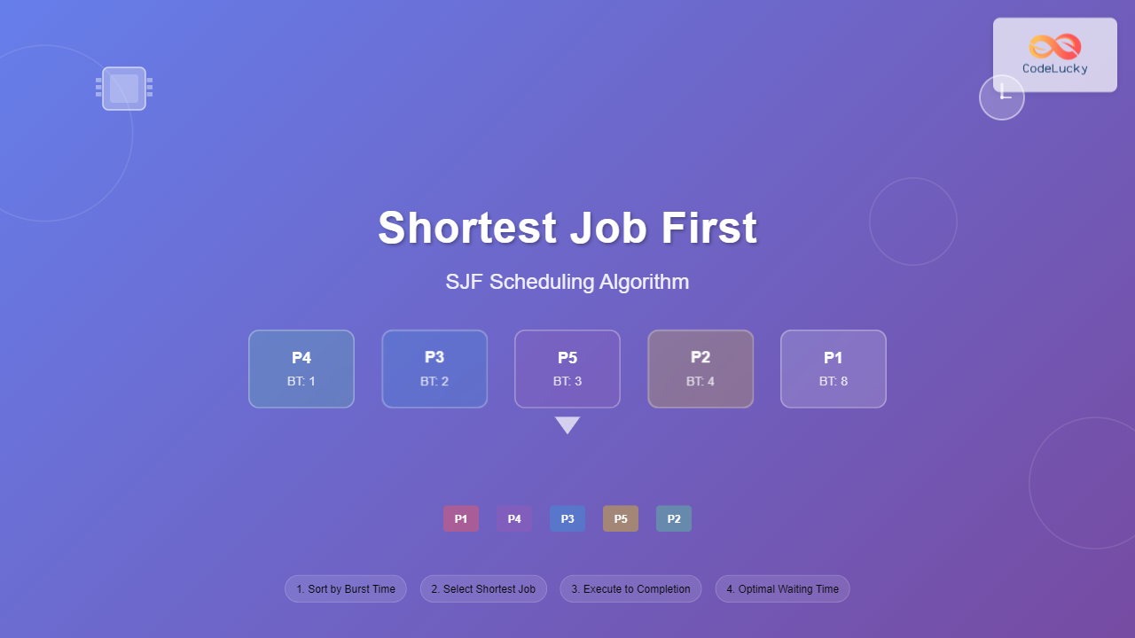
Shortest Job First (SJF) scheduling is a CPU scheduling algorithm that selects the process with the smallest execution time (burst time) for execution next. This algorithm aims to minimize the average waiting time for all processes in the system, making it one of the most optimal scheduling algorithms in terms of waiting time.
SJF scheduling operates on a simple principle: among all available processes, always execute the one that requires the least amount of CPU time. This greedy approach leads to optimal average waiting time, though it comes with certain practical challenges.
Types of SJF Scheduling
1. Non-Preemptive SJF
In non-preemptive SJF, once a process starts execution, it cannot be interrupted until it completes. The scheduler only makes decisions when:
- The currently running process finishes execution
- A new process arrives in the ready queue
2. Preemptive SJF (Shortest Remaining Time First – SRTF)
Preemptive SJF, also known as Shortest Remaining Time First (SRTF), allows the scheduler to interrupt a currently running process if a new process arrives with a shorter burst time than the remaining time of the current process.
SJF Algorithm Implementation
Non-Preemptive SJF Algorithm
Algorithm: Non-Preemptive SJF
1. Sort processes by arrival time
2. At time t=0, select the process with shortest burst time among arrived processes
3. Execute the selected process to completion
4. When process completes, select next shortest job among available processes
5. Repeat until all processes are completed

Pseudocode:
while (processes remaining):
    available_processes = processes with arrival_time <= current_time
    if available_processes is empty:
        current_time = next earliest arrival_time
        continue

    shortest_job = process with minimum burst_time in available_processes
    execute(shortest_job)
    current_time += shortest_job.burst_time
    calculate_times(shortest_job)
    remove(shortest_job from process_list)
Preemptive SJF Algorithm
Algorithm: Preemptive SJF (SRTF)
1. At each time unit, check for newly arrived processes
2. Among all available processes (including currently running), select the one with shortest remaining time
3. If the selected process is different from currently running process, perform context switch
4. Execute for one time unit and update remaining time
5. Repeat until all processes complete

Pseudocode:
current_time = 0
while (processes remaining):
    available_processes = processes with arrival_time <= current_time
    if available_processes is empty:
        current_time++
        continue

    shortest_remaining = process with minimum remaining_time in available_processes
    if shortest_remaining != current_process:
        context_switch(shortest_remaining)

    execute(shortest_remaining, 1)
    shortest_remaining.remaining_time--
    current_time++

    if shortest_remaining.remaining_time == 0:
        calculate_completion_time(shortest_remaining)
Detailed Example: Non-Preemptive SJF
Let’s work through a comprehensive example with five processes:
| Process | Arrival Time | Burst Time |
|---|---|---|
| P1 | 0 | 8 |
| P2 | 1 | 4 |
| P3 | 2 | 2 |
| P4 | 3 | 1 |
| P5 | 4 | 3 |
Step-by-Step Execution
Execution Analysis:
- Time 0-8: P1 starts execution (only available process)
- Time 8: P1 completes. Available processes: P2(4), P3(2), P4(1), P5(3). Select P4 (shortest)
- Time 9: P4 completes. Available processes: P2(4), P3(2), P5(3). Select P3 (shortest)
- Time 11: P3 completes. Available processes: P2(4), P5(3). Select P5 (shortest)
- Time 14: P5 completes. Available processes: P2(4). Select P2
- Time 18: P2 completes. All processes finished
Time Calculations
| Process | Arrival Time | Burst Time | Completion Time | Turnaround Time | Waiting Time |
|---|---|---|---|---|---|
| P1 | 0 | 8 | 8 | 8 | 0 |
| P2 | 1 | 4 | 18 | 17 | 13 |
| P3 | 2 | 2 | 11 | 9 | 7 |
| P4 | 3 | 1 | 9 | 6 | 5 |
| P5 | 4 | 3 | 14 | 10 | 7 |
Performance Metrics:
- Average Turnaround Time = (8 + 17 + 9 + 6 + 10) / 5 = 10 units
- Average Waiting Time = (0 + 13 + 7 + 5 + 7) / 5 = 6.4 units
Detailed Example: Preemptive SJF (SRTF)
Using the same processes but with preemptive scheduling:
Step-by-Step Preemptive Execution
- Time 0-1: P1 executes (remaining: 7)
- Time 1: P2 arrives (BT=4). P2 < P1’s remaining time (7), so preempt P1
- Time 1-2: P2 executes (remaining: 3)
- Time 2: P3 arrives (BT=2). P3 < P2’s remaining time (3), so preempt P2
- Time 2-3: P3 executes (remaining: 1)
- Time 3: P4 arrives (BT=1). P4 = P3’s remaining time, continue P3
- Time 3-4: P3 completes. P4 has shortest time (1)
- Time 4: P4 completes. P5 arrives (BT=3)
- Time 4-5: P5 executes and completes
- Time 5-13: P1 resumes and completes
- Time 13-17: P2 resumes and completes
| Process | Arrival Time | Burst Time | Completion Time | Turnaround Time | Waiting Time |
|---|---|---|---|---|---|
| P1 | 0 | 8 | 13 | 13 | 5 |
| P2 | 1 | 4 | 17 | 16 | 12 |
| P3 | 2 | 2 | 4 | 2 | 0 |
| P4 | 3 | 1 | 5 | 2 | 1 |
| P5 | 4 | 3 | 8 | 4 | 1 |
Preemptive SJF Performance:
- Average Turnaround Time = (13 + 16 + 2 + 2 + 4) / 5 = 7.4 units
- Average Waiting Time = (5 + 12 + 0 + 1 + 1) / 5 = 3.8 units
Advantages of SJF Scheduling
- Optimal Average Waiting Time: SJF provides the minimum average waiting time among all scheduling algorithms
- Efficient Resource Utilization: Shorter jobs complete quickly, freeing up system resources
- Reduced System Load: Faster completion of processes reduces the number of processes in the system
- Better Response Time: Short jobs get executed quickly, improving user experience
Disadvantages of SJF Scheduling
- Starvation Problem: Long processes may wait indefinitely if short processes keep arriving
- Burst Time Prediction: Difficult to know exact execution time in advance in real systems
- Context Switching Overhead: Preemptive SJF may cause frequent context switches
- Not Suitable for Interactive Systems: May not provide good response times for interactive processes
SJF vs Other Scheduling Algorithms
| Algorithm | Average Waiting Time | Starvation | Preemption | Implementation |
|---|---|---|---|---|
| FCFS | High | No | No | Simple |
| SJF (Non-preemptive) | Optimal | Yes | No | Moderate |
| SJF (Preemptive) | Better than Non-preemptive | Yes | Yes | Complex |
| Round Robin | Moderate | No | Yes | Simple |
| Priority | Depends on Priority | Yes | Optional | Moderate |
Burst Time Prediction Techniques
Since exact burst time is unknown in real systems, various prediction methods are used:
Exponential Averaging
τ(n+1) = α × t(n) + (1-α) × τ(n)

Where:
- τ(n+1) = Predicted burst time for next CPU burst
- t(n) = Actual burst time of nth CPU burst
- τ(n) = Predicted burst time for nth CPU burst
- α = Smoothing factor (0 ≤ α ≤ 1)

Example:
If α = 0.5, t(1) = 10, τ(1) = 8
τ(2) = 0.5 × 10 + 0.5 × 8 = 9
Historical Analysis
- Simple Average: Average of previous burst times
- Weighted Average: More weight to recent bursts
- Process Classification: Group similar processes and use their average
Real-World Applications and Modifications
Aging Technique to Prevent Starvation
Algorithm: SJF with Aging
1. Assign initial priority based on burst time
2. Increase priority of waiting processes over time
3. Select process with highest priority (considering both burst time and waiting time)

Priority = Base_Priority + (Waiting_Time / Aging_Factor)

Where Base_Priority is inversely proportional to burst time
Multi-Level Queue with SJF
Combine SJF with other algorithms:
- Interactive Queue: Use Round Robin for interactive processes
- Batch Queue: Use SJF for batch processes
- System Queue: High priority for system processes
Implementation Example in C++
#include <iostream>
#include <vector>
#include <algorithm>
#include <queue>

struct Process {
    int id;
    int arrival_time;
    int burst_time;
    int remaining_time;
    int completion_time;
    int waiting_time;
    int turnaround_time;

    Process(int i, int at, int bt) :
        id(i), arrival_time(at), burst_time(bt), remaining_time(bt) {}
};

class SJFScheduler {
private:
    std::vector<Process> processes;

public:
    void addProcess(int id, int arrival_time, int burst_time) {
        processes.emplace_back(id, arrival_time, burst_time);
    }

    void nonPreemptiveSJF() {
        std::sort(processes.begin(), processes.end(),
                 [](const Process& a, const Process& b) {
                     return a.arrival_time < b.arrival_time;
                 });

        std::vector<bool> completed(processes.size(), false);
        int current_time = 0;
        int completed_count = 0;

        while (completed_count < processes.size()) {
            int shortest_idx = -1;
            int shortest_burst = INT_MAX;

            // Find shortest job among arrived processes
            for (int i = 0; i < processes.size(); i++) {
                if (!completed[i] &&
                    processes[i].arrival_time <= current_time &&
                    processes[i].burst_time < shortest_burst) {
                    shortest_burst = processes[i].burst_time;
                    shortest_idx = i;
                }
            }

            if (shortest_idx == -1) {
                current_time++;
                continue;
            }

            // Execute the shortest job
            current_time += processes[shortest_idx].burst_time;
            processes[shortest_idx].completion_time = current_time;
            processes[shortest_idx].turnaround_time =
                current_time - processes[shortest_idx].arrival_time;
            processes[shortest_idx].waiting_time =
                processes[shortest_idx].turnaround_time -
                processes[shortest_idx].burst_time;

            completed[shortest_idx] = true;
            completed_count++;
        }
    }

    void displayResults() {
        std::cout << "Process\tAT\tBT\tCT\tTAT\tWT\n";
        double total_tat = 0, total_wt = 0;

        for (const auto& p : processes) {
            std::cout << "P" << p.id << "\t"
                     << p.arrival_time << "\t"
                     << p.burst_time << "\t"
                     << p.completion_time << "\t"
                     << p.turnaround_time << "\t"
                     << p.waiting_time << "\n";

            total_tat += p.turnaround_time;
            total_wt += p.waiting_time;
        }

        std::cout << "\nAverage Turnaround Time: "
                 << total_tat / processes.size() << std::endl;
        std::cout << "Average Waiting Time: "
                 << total_wt / processes.size() << std::endl;
    }
};
Performance Analysis and Complexity
Time Complexity
- Non-preemptive SJF: O(n²) for each scheduling decision
- Preemptive SJF: O(n²) for each time unit
- With Priority Queue: O(n log n) for sorting and O(log n) for each insertion/deletion
Space Complexity
- Basic Implementation: O(n) for storing process information
- With Additional Data Structures: O(n) for ready queue and process tracking
Best Practices and Optimization
Implementation Optimizations
- Use Priority Queues: Implement ready queue as a min-heap based on burst time
- Efficient Process Selection: Maintain sorted order to avoid repeated searching
- Batch Processing: Group processes with similar characteristics
- Hybrid Approaches: Combine SJF with other algorithms for specific use cases
Practical Considerations
- Process Classification: Categorize processes as CPU-bound or I/O-bound
- Dynamic Adjustment: Adapt burst time predictions based on system load
- User Interface: Provide different scheduling for interactive vs. batch processes
- System Monitoring: Track algorithm performance and adjust parameters
Conclusion
Shortest Job First scheduling is a powerful algorithm that provides optimal average waiting time, making it highly efficient for batch processing systems. While it faces challenges like starvation and burst time prediction in real-world scenarios, various modifications and hybrid approaches can address these limitations.
Understanding SJF is crucial for system administrators, operating system designers, and anyone working with process scheduling. The algorithm’s principles apply beyond operating systems to various resource allocation problems in computer science and distributed systems.
When implementing SJF, consider the specific requirements of your system, the nature of processes, and the trade-offs between optimality and fairness. Combining SJF with aging mechanisms or multi-level queue structures can provide the benefits of optimal scheduling while maintaining system responsiveness and preventing starvation.

