What is Round Robin Scheduling?
Round Robin (RR) scheduling is a preemptive CPU scheduling algorithm that assigns equal time slices, called time quantum or time slice, to each process in a circular queue. It’s one of the most widely used scheduling algorithms in modern operating systems due to its fairness and simplicity.
The algorithm operates on a simple principle: each process gets an equal opportunity to execute for a fixed time period. When a process’s time quantum expires, it’s moved to the back of the ready queue, and the next process gets CPU access.

Key Components of Round Robin Scheduling
Time Quantum (Time Slice)
The time quantum is the most critical parameter in Round Robin scheduling. It determines how long each process can execute before being preempted. The choice of time quantum significantly impacts system performance:
- Small Time Quantum: Better response time but higher context switching overhead
- Large Time Quantum: Reduced overhead but may lead to poor response time
- Optimal Time Quantum: Balances response time and system efficiency
Ready Queue Structure
Round Robin uses a circular queue (First-In-First-Out) to maintain processes. New processes are added to the tail, and the scheduler picks processes from the head.

Round Robin Algorithm Implementation
Algorithm Steps
- Initialize the ready queue with all processes
- Set the time quantum value
- Select the first process from the queue
- Execute the process for the time quantum duration
- If process completes within time quantum, remove it from queue
- If time quantum expires, move process to end of queue
- Repeat until all processes complete
Pseudocode Implementation
ALGORITHM: Round Robin Scheduling
INPUT: Process array, Time Quantum
OUTPUT: Execution order, waiting times, turnaround times

BEGIN
    Initialize ready_queue as circular queue
    SET current_time = 0

    WHILE ready_queue is not empty DO
        process = ready_queue.front()
        ready_queue.dequeue()

        IF process.remaining_time <= time_quantum THEN
            current_time += process.remaining_time
            process.completion_time = current_time
            process.turnaround_time = completion_time - arrival_time
            process.waiting_time = turnaround_time - burst_time
        ELSE
            current_time += time_quantum
            process.remaining_time -= time_quantum
            ready_queue.enqueue(process)
        END IF
    END WHILE
END
Practical Example: Round Robin Execution
Let’s analyze a comprehensive example with five processes to understand Round Robin scheduling behavior:
| Process | Arrival Time | Burst Time | Priority |
|---|---|---|---|
| P1 | 0 | 8 | 3 |
| P2 | 1 | 4 | 1 |
| P3 | 2 | 9 | 4 |
| P4 | 3 | 5 | 2 |
| P5 | 4 | 2 | 5 |
Time Quantum = 3
Execution Timeline

Step-by-Step Execution
Time 0-3: P1 executes (remaining: 5), P2, P3, P4 arrive
Time 3-6: P2 executes (remaining: 1), P5 arrives
Time 6-9: P3 executes (remaining: 6)
Time 9-12: P4 executes (remaining: 2)
Time 12-14: P5 completes (remaining: 0)
Time 14-17: P1 executes (remaining: 2)
Time 17-19: P2 completes (remaining: 0)
Time 19-22: P3 executes (remaining: 3)
Time 22-24: P4 completes (remaining: 0)
Time 24-26: P1 completes (remaining: 0)
Time 26-29: P3 completes (remaining: 0)
Performance Metrics Calculation
| Process | Completion Time | Turnaround Time | Waiting Time | Response Time |
|---|---|---|---|---|
| P1 | 26 | 26 | 18 | 0 |
| P2 | 19 | 18 | 14 | 2 |
| P3 | 29 | 27 | 18 | 4 |
| P4 | 24 | 21 | 16 | 6 |
| P5 | 14 | 10 | 8 | 8 |
Average Turnaround Time: (26 + 18 + 27 + 21 + 10) / 5 = 20.4
Average Waiting Time: (18 + 14 + 18 + 16 + 8) / 5 = 14.8
Average Response Time: (0 + 2 + 4 + 6 + 8) / 5 = 4.0
Time Quantum Impact Analysis
Performance Comparison with Different Time Quantum Values
Using the same process set, let’s compare performance with different time quantum values:
| Time Quantum | Avg Turnaround Time | Avg Waiting Time | Context Switches | Response Time |
|---|---|---|---|---|
| 1 | 22.6 | 17.0 | 18 | 2.0 |
| 2 | 21.2 | 15.6 | 12 | 3.0 |
| 3 | 20.4 | 14.8 | 9 | 4.0 |
| 4 | 19.8 | 14.2 | 7 | 5.0 |
| 5 | 19.4 | 13.8 | 6 | 6.0 |

Advantages of Round Robin Scheduling
- Fairness: Every process gets equal CPU time allocation
- No Starvation: All processes eventually get CPU access
- Good Response Time: Interactive processes receive quick response
- Simple Implementation: Easy to understand and implement
- Preemptive: Prevents long processes from monopolizing CPU
- Time Sharing: Ideal for multi-user and interactive systems
Disadvantages and Limitations
- Context Switching Overhead: Frequent switches consume system resources
- Poor for Batch Jobs: Not optimal for CPU-intensive processes
- Time Quantum Dependency: Performance heavily depends on quantum selection
- Average Waiting Time: Often higher than other algorithms
- No Priority Consideration: Treats all processes equally regardless of importance
Optimization Strategies
Dynamic Time Quantum Adjustment
Modern implementations use adaptive time quantum that adjusts based on system load and process characteristics:
- Load-based Adjustment: Increase quantum during low load, decrease during high load
- Process-type Awareness: Different quantum for I/O-bound vs CPU-bound processes
- Historical Analysis: Adjust based on past execution patterns
Hybrid Approaches
Combining Round Robin with other scheduling algorithms:
- Multi-level Queue: Different queues with different time quantum values
- Priority Round Robin: Incorporate priority levels with round robin within each level
- Shortest Remaining Time + RR: Switch algorithms based on process characteristics
Real-world Applications
Operating Systems Using Round Robin
- Linux: Completely Fair Scheduler (CFS) incorporates RR concepts
- Windows: Uses round robin for threads at the same priority level
- Unix: Traditional Unix systems use RR for time-sharing
- Embedded Systems: Real-time systems often use modified RR
Time Quantum Selection Guidelines
Choosing optimal time quantum depends on several factors:
| System Type | Recommended Quantum | Reasoning |
|---|---|---|
| Interactive Systems | 10-100ms | Good response time for user interaction |
| Server Systems | 100-500ms | Balance between throughput and responsiveness |
| Batch Systems | 500ms-2s | Minimize context switching overhead |
| Real-time Systems | 1-10ms | Meet strict timing requirements |
Performance Analysis Techniques
Key Performance Metrics
When analyzing Round Robin performance, focus on these critical metrics:
- Turnaround Time: Total time from arrival to completion
- Waiting Time: Time spent in ready queue
- Response Time: Time from arrival to first execution
- Context Switch Count: Number of process switches
- CPU Utilization: Percentage of time CPU is busy
- Throughput: Number of processes completed per unit time
Benchmark Testing
For comprehensive performance analysis, test Round Robin with:
- Varying Process Mix: Different ratios of CPU-bound and I/O-bound processes
- Different Arrival Patterns: Uniform, bursty, and random arrivals
- Multiple Time Quantum Values: Find optimal quantum for specific workloads
- System Load Variations: Test under different load conditions
Advanced Round Robin Variants
Multilevel Feedback Queue
This sophisticated approach uses multiple Round Robin queues with different priorities and time quantum values, allowing processes to move between queues based on their behavior.
Weighted Round Robin
Assigns different weights to processes, allowing some processes to receive larger time slices or more frequent scheduling opportunities.
Deficit Round Robin
Tracks “deficit” for each process to ensure fair allocation over time, particularly useful in network scheduling and resource allocation.
Implementation Considerations
Data Structures
Efficient Round Robin implementation requires:
- Circular Queue: For maintaining process order
- Process Control Blocks: Store process state and timing information
- Timer Interrupt Handler: Manage time quantum expiration
- Context Switch Mechanism: Save/restore process state efficiently
System Integration
Round Robin scheduling must integrate with:
- Memory Management: Handle page faults during context switches
- I/O Subsystem: Manage blocked processes effectively
- Interrupt Handling: Maintain scheduling integrity during interrupts
- Load Balancing: Distribute processes across multiple CPUs in SMP systems
Round Robin scheduling remains a fundamental algorithm in operating systems, providing an excellent balance between fairness, simplicity, and performance. Understanding its time quantum behavior and performance characteristics is essential for system administrators, developers, and anyone working with multi-tasking environments. The key to successful Round Robin implementation lies in careful time quantum selection and consideration of the specific system requirements and workload characteristics.
Related Posts
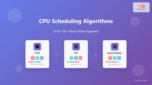
CPU Scheduling Algorithms: FCFS, SJF, Round Robin Complete Guide
CPU scheduling is a fundamental concept in operating systems that determines how processes are allocated processor time. The CPU scheduler...
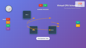
Virtual CPU Scheduling: Complete Guide to Time-sharing Physical Processors
Virtual CPU scheduling is the cornerstone of modern operating systems, enabling multiple processes to share limited physical processors efficiently. This...
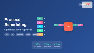
Process Scheduling in Operating System: Algorithms, Types & Implementation Guide
Process scheduling is one of the most critical components of an operating system that determines how the CPU time is...
Multilevel Queue Scheduling: Multiple Priority Levels in Operating Systems
Introduction to Multilevel Queue Scheduling Multilevel queue scheduling is a sophisticated CPU scheduling algorithm used in operating systems to manage...

Priority Scheduling Algorithm: Complete Implementation Guide with Examples
What is Priority Scheduling Algorithm? Priority scheduling is a CPU scheduling algorithm where each process is assigned a priority value,...

Preemptive vs Non-Preemptive Scheduling: Complete Guide to CPU Scheduling in Operating Systems
Understanding CPU Scheduling in Operating Systems CPU scheduling is one of the most critical functions of an operating system, determining...

Shortest Job First Scheduling: SJF Algorithm Explained with Examples and Implementation
What is Shortest Job First (SJF) Scheduling? Shortest Job First (SJF) scheduling is a CPU scheduling algorithm that selects the...

Completely Fair Scheduler: Linux CFS Algorithm Deep Dive
The Linux Completely Fair Scheduler (CFS) revolutionized process scheduling in the Linux kernel when it was introduced in version 2.6.23....

Fair Share Scheduling: Resource Allocation by User Groups in Operating Systems
Introduction to Fair Share Scheduling Fair Share Scheduling (FSS) is a sophisticated CPU scheduling algorithm designed to allocate computing resources...

Lottery Scheduling: Fair CPU Allocation Through Proportional Sharing
Introduction to Lottery Scheduling Lottery scheduling is a probabilistic CPU scheduling algorithm that provides proportional share resource allocation by assigning...
Thread in Operating System: Lightweight Processes and Multithreading Explained
What are Threads in Operating Systems? A thread is the smallest unit of execution within a process that can be...

Device Scheduling: Complete Guide to I/O Request Scheduling Algorithms
Device scheduling is a critical component of operating system design that determines how I/O requests are ordered and executed to...
- What is Round Robin Scheduling?
- Key Components of Round Robin Scheduling
- Round Robin Algorithm Implementation
- Practical Example: Round Robin Execution
- Time Quantum Impact Analysis
- Advantages of Round Robin Scheduling
- Disadvantages and Limitations
- Optimization Strategies
- Real-world Applications
- Performance Analysis Techniques
- Advanced Round Robin Variants
- Implementation Considerations