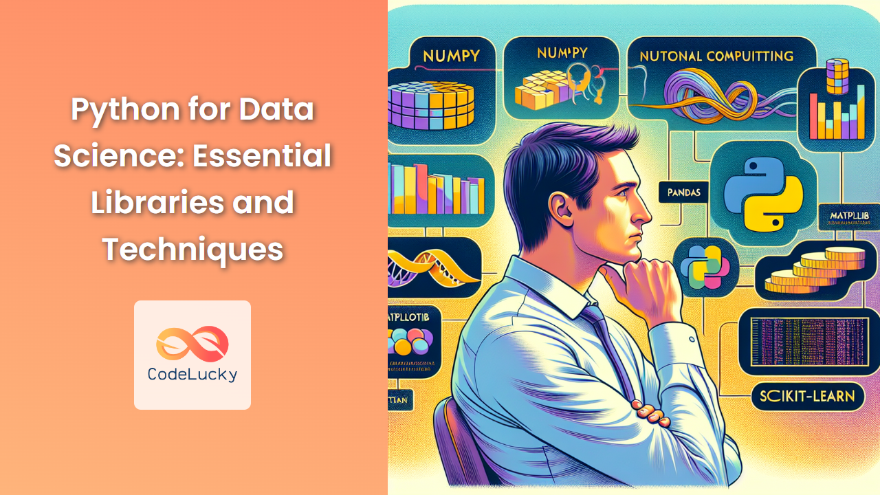
Python has become the go-to language for data scientists worldwide, thanks to its simplicity, versatility, and robust ecosystem of libraries. In this comprehensive guide, we'll explore the essential Python libraries and techniques that every data scientist should master. We'll dive deep into practical examples, demonstrating how to leverage these tools to extract insights from data effectively.

NumPy: The Foundation of Scientific Computing

NumPy (Numerical Python) is the cornerstone of scientific computing in Python. It provides support for large, multi-dimensional arrays and matrices, along with a vast collection of mathematical functions to operate on these arrays efficiently.

Creating and Manipulating Arrays

Let's start with the basics of creating and manipulating NumPy arrays:

import numpy as np

# Create a 1D array
arr1d = np.array([1, 2, 3, 4, 5])
print("1D Array:", arr1d)

# Create a 2D array
arr2d = np.array([[1, 2, 3], [4, 5, 6], [7, 8, 9]])
print("2D Array:\n", arr2d)

# Array operations
print("Array sum:", arr1d.sum())
print("Array mean:", arr1d.mean())
print("Array standard deviation:", arr1d.std())

# Element-wise operations
print("Element-wise multiplication:", arr1d * 2)
print("Element-wise addition:", arr1d + 5)

# Reshaping arrays
reshaped_arr = arr1d.reshape(5, 1)
print("Reshaped array:\n", reshaped_arr)

This example demonstrates the creation of 1D and 2D arrays, basic array operations, element-wise operations, and reshaping arrays. These operations are fundamental to data manipulation in scientific computing.

Broadcasting in NumPy

Broadcasting is a powerful feature in NumPy that allows operations between arrays of different shapes. Let's see it in action:

# Broadcasting example
a = np.array([1, 2, 3])
b = np.array([[1], [2], [3]])

print("Array a shape:", a.shape)
print("Array b shape:", b.shape)

result = a + b
print("Result of a + b:\n", result)
print("Result shape:", result.shape)

In this example, NumPy automatically broadcasts the 1D array a across the columns of the 2D array b, allowing element-wise addition despite their different shapes.

Pandas: Data Manipulation and Analysis

Pandas is a powerful library for data manipulation and analysis. It provides data structures like DataFrames and Series that make working with structured data intuitive and efficient.

Creating and Manipulating DataFrames

Let's explore some basic operations with Pandas DataFrames:

import pandas as pd

# Create a DataFrame
data = {
    'Name': ['Alice', 'Bob', 'Charlie', 'David'],
    'Age': [25, 30, 35, 28],
    'City': ['New York', 'San Francisco', 'Los Angeles', 'Chicago']
}
df = pd.DataFrame(data)
print("Original DataFrame:\n", df)

# Accessing columns
print("\nNames:\n", df['Name'])

# Adding a new column
df['Salary'] = [50000, 60000, 75000, 55000]
print("\nDataFrame with new column:\n", df)

# Filtering data
young_people = df[df['Age'] < 30]
print("\nPeople younger than 30:\n", young_people)

# Grouping and aggregation
avg_salary_by_city = df.groupby('City')['Salary'].mean()
print("\nAverage salary by city:\n", avg_salary_by_city)

This example shows how to create a DataFrame, access columns, add new columns, filter data based on conditions, and perform grouping and aggregation operations.

Handling Missing Data

Dealing with missing data is a common task in data science. Pandas provides several methods to handle missing values:

# Create a DataFrame with missing values
data_with_nan = {
    'A': [1, 2, np.nan, 4],
    'B': [5, np.nan, np.nan, 8],
    'C': [9, 10, 11, 12]
}
df_nan = pd.DataFrame(data_with_nan)
print("DataFrame with NaN values:\n", df_nan)

# Check for missing values
print("\nMissing values:\n", df_nan.isnull())

# Fill missing values
df_filled = df_nan.fillna(0)
print("\nDataFrame with NaN replaced by 0:\n", df_filled)

# Drop rows with any NaN values
df_dropped = df_nan.dropna()
print("\nDataFrame with NaN rows dropped:\n", df_dropped)

This example demonstrates how to identify missing values, fill them with a specific value, and drop rows containing missing data.

Matplotlib: Data Visualization

Matplotlib is the most widely used library for creating static, animated, and interactive visualizations in Python. Let's explore some basic plotting techniques:

Line Plots and Scatter Plots

import matplotlib.pyplot as plt

# Generate some data
x = np.linspace(0, 10, 100)
y1 = np.sin(x)
y2 = np.cos(x)

# Create a line plot
plt.figure(figsize=(10, 5))
plt.plot(x, y1, label='sin(x)')
plt.plot(x, y2, label='cos(x)')
plt.title('Sine and Cosine Functions')
plt.xlabel('x')
plt.ylabel('y')
plt.legend()
plt.grid(True)
plt.show()

# Create a scatter plot
plt.figure(figsize=(10, 5))
plt.scatter(x, y1, c=y2, cmap='viridis')
plt.colorbar(label='cos(x)')
plt.title('Scatter Plot of sin(x) colored by cos(x)')
plt.xlabel('x')
plt.ylabel('sin(x)')
plt.show()

This example creates a line plot showing sine and cosine functions, and a scatter plot of sine values colored by cosine values.

Bar Plots and Histograms

# Bar plot
categories = ['A', 'B', 'C', 'D']
values = [4, 7, 2, 8]

plt.figure(figsize=(8, 5))
plt.bar(categories, values)
plt.title('Bar Plot Example')
plt.xlabel('Categories')
plt.ylabel('Values')
plt.show()

# Histogram
data = np.random.randn(1000)

plt.figure(figsize=(8, 5))
plt.hist(data, bins=30, edgecolor='black')
plt.title('Histogram of Random Data')
plt.xlabel('Value')
plt.ylabel('Frequency')
plt.show()

This example demonstrates how to create a bar plot and a histogram using Matplotlib.

Scikit-learn: Machine Learning in Python

Scikit-learn is a powerful library for machine learning in Python. It provides simple and efficient tools for data mining and data analysis. Let's explore some basic machine learning tasks using scikit-learn:

Linear Regression

from sklearn.model_selection import train_test_split
from sklearn.linear_model import LinearRegression
from sklearn.metrics import mean_squared_error, r2_score

# Generate sample data
X = np.array([[1], [2], [3], [4], [5]])
y = np.array([2, 4, 5, 4, 5])

# Split the data into training and testing sets
X_train, X_test, y_train, y_test = train_test_split(X, y, test_size=0.2, random_state=42)

# Create and train the model
model = LinearRegression()
model.fit(X_train, y_train)

# Make predictions
y_pred = model.predict(X_test)

# Evaluate the model
mse = mean_squared_error(y_test, y_pred)
r2 = r2_score(y_test, y_pred)

print("Mean squared error: ", mse)
print("R-squared score: ", r2)

# Visualize the results
plt.scatter(X, y, color='blue', label='Data points')
plt.plot(X, model.predict(X), color='red', label='Linear regression')
plt.title('Linear Regression Example')
plt.xlabel('X')
plt.ylabel('y')
plt.legend()
plt.show()

This example demonstrates how to perform linear regression using scikit-learn, including data splitting, model training, prediction, and evaluation.

Classification with K-Nearest Neighbors

from sklearn.neighbors import KNeighborsClassifier
from sklearn.datasets import load_iris
from sklearn.metrics import accuracy_score, classification_report

# Load the Iris dataset
iris = load_iris()
X, y = iris.data, iris.target

# Split the data
X_train, X_test, y_train, y_test = train_test_split(X, y, test_size=0.3, random_state=42)

# Create and train the model
knn = KNeighborsClassifier(n_neighbors=3)
knn.fit(X_train, y_train)

# Make predictions
y_pred = knn.predict(X_test)

# Evaluate the model
accuracy = accuracy_score(y_test, y_pred)
print("Accuracy:", accuracy)
print("\nClassification Report:\n", classification_report(y_test, y_pred, target_names=iris.target_names))

# Visualize the results (for 2 features)
plt.figure(figsize=(10, 6))
plt.scatter(X[:, 0], X[:, 1], c=y, cmap='viridis')
plt.title('Iris Dataset - Sepal Length vs Sepal Width')
plt.xlabel('Sepal Length (cm)')
plt.ylabel('Sepal Width (cm)')
plt.colorbar(label='Species')
plt.show()

This example shows how to perform classification using the K-Nearest Neighbors algorithm on the Iris dataset, including model training, prediction, evaluation, and visualization.

Advanced Techniques: Working with Big Data

When dealing with large datasets that don't fit into memory, you need to use specialized tools and techniques. Let's explore some options:

Dask: Parallel Computing

Dask is a flexible library for parallel computing in Python. It's particularly useful for working with large datasets:

import dask.dataframe as dd

# Create a large Dask DataFrame
df = dd.read_csv('large_dataset.csv')  # Assume we have a large CSV file

# Perform operations on the Dask DataFrame
result = df.groupby('category').agg({'value': ['mean', 'sum']})

# Compute the result
final_result = result.compute()

print(final_result)

This example demonstrates how to use Dask to read and process a large CSV file that doesn't fit into memory.

PySpark: Distributed Computing

PySpark is the Python API for Apache Spark, a powerful engine for large-scale data processing:

from pyspark.sql import SparkSession
from pyspark.sql.functions import col, avg

# Create a SparkSession
spark = SparkSession.builder.appName("BigDataProcessing").getOrCreate()

# Read a large dataset
df = spark.read.csv("huge_dataset.csv", header=True, inferSchema=True)

# Perform operations
result = df.groupBy("category").agg(avg("value").alias("avg_value"))

# Show the result
result.show()

# Stop the SparkSession
spark.stop()

This example shows how to use PySpark to process a large dataset distributed across a cluster of computers.

Conclusion

Python's rich ecosystem of data science libraries provides powerful tools for every stage of the data science workflow, from data manipulation and analysis to visualization and machine learning. By mastering these essential libraries and techniques, you'll be well-equipped to tackle a wide range of data science challenges.

Remember, the key to becoming proficient in data science with Python is practice. Experiment with these libraries using your own datasets, and don't hesitate to explore the extensive documentation available for each library to discover more advanced features and techniques.

As you continue your journey in data science, you'll find that these libraries form the foundation upon which you can build more complex and sophisticated data analysis and machine learning projects. Happy coding, and may your data always yield valuable insights! 🐍📊🧠