Process scheduling is one of the most critical components of an operating system that determines how the CPU time is allocated among competing processes. It directly impacts system performance, response time, and resource utilization. Understanding process scheduling algorithms is essential for system administrators, developers, and anyone working with operating systems.
What is Process Scheduling?
Process scheduling is the mechanism by which an operating system decides which process should be executed by the CPU at any given time. When multiple processes compete for CPU resources, the scheduler must make intelligent decisions to optimize system performance while ensuring fairness and meeting various quality of service requirements.
The primary objectives of process scheduling include:
- CPU Utilization: Maximize the percentage of time the CPU is busy executing processes
- Throughput: Maximize the number of processes completed per unit time
- Turnaround Time: Minimize the total time from process submission to completion
- Waiting Time: Minimize the time processes spend waiting in the ready queue
- Response Time: Minimize the time from request submission to first response
- Fairness: Ensure all processes get reasonable access to CPU resources
Process States and Scheduling Context
Before diving into scheduling algorithms, it’s crucial to understand process states and how they relate to scheduling decisions.

The scheduler primarily works with processes in the Ready state, selecting which process should transition to the Running state. This decision-making process is where different scheduling algorithms come into play.
Types of Scheduling
1. Preemptive vs Non-Preemptive Scheduling
Preemptive Scheduling: The operating system can forcibly remove a process from the CPU before it completes execution. This allows for better responsiveness and prevents any single process from monopolizing the CPU.
Non-Preemptive Scheduling: Once a process starts execution, it continues until it voluntarily gives up the CPU (either by completing or requesting I/O operations).
2. Short-term, Medium-term, and Long-term Scheduling
- Long-term Scheduler: Determines which processes are admitted to the system
- Medium-term Scheduler: Handles swapping processes between main memory and storage
- Short-term Scheduler: Makes frequent decisions about which ready process should execute next
Major CPU Scheduling Algorithms
1. First-Come, First-Served (FCFS)
FCFS is the simplest scheduling algorithm where processes are executed in the order they arrive in the ready queue. It’s non-preemptive and follows a strict first-in-first-out policy.
Example:
| Process | Arrival Time | Burst Time | Start Time | Completion Time | Turnaround Time | Waiting Time |
|---|---|---|---|---|---|---|
| P1 | 0 | 4 | 0 | 4 | 4 | 0 |
| P2 | 1 | 3 | 4 | 7 | 6 | 3 |
| P3 | 2 | 2 | 7 | 9 | 7 | 5 |
| P4 | 3 | 1 | 9 | 10 | 7 | 6 |
Average Turnaround Time: (4 + 6 + 7 + 7) / 4 = 6 units
Average Waiting Time: (0 + 3 + 5 + 6) / 4 = 3.5 units
Advantages:
- Simple to understand and implement
- No starvation – every process eventually gets executed
- Fair in terms of arrival order
Disadvantages:
- Can lead to convoy effect (short processes wait for long processes)
- Poor average waiting time
- Not suitable for interactive systems
2. Shortest Job First (SJF)
SJF selects the process with the shortest burst time for execution. It can be implemented as both preemptive (Shortest Remaining Time First) and non-preemptive versions.
Non-Preemptive SJF Example:
| Process | Arrival Time | Burst Time | Start Time | Completion Time | Turnaround Time | Waiting Time |
|---|---|---|---|---|---|---|
| P1 | 0 | 4 | 3 | 7 | 7 | 3 |
| P2 | 1 | 3 | 0 | 3 | 2 | -1 |
| P3 | 2 | 2 | 7 | 9 | 7 | 5 |
| P4 | 3 | 1 | 9 | 10 | 7 | 6 |
Execution Order: P2 → P1 → P3 → P4
Advantages:
- Optimal average waiting time
- Better throughput compared to FCFS
- Minimizes average turnaround time
Disadvantages:
- Can cause starvation of long processes
- Requires knowledge of burst times in advance
- Not practical for interactive systems
3. Round Robin (RR)
Round Robin is a preemptive algorithm that assigns a fixed time quantum to each process. If a process doesn’t complete within its quantum, it’s preempted and moved to the end of the ready queue.

Example with Time Quantum = 2:
| Process | Arrival Time | Burst Time | Completion Time | Turnaround Time | Waiting Time |
|---|---|---|---|---|---|
| P1 | 0 | 4 | 8 | 8 | 4 |
| P2 | 1 | 3 | 9 | 8 | 5 |
| P3 | 2 | 2 | 6 | 4 | 2 |
| P4 | 3 | 1 | 7 | 4 | 3 |
Execution Timeline: P1(0-2) → P2(2-4) → P3(4-6) → P4(6-7) → P1(7-8) → P2(8-9)
Advantages:
- Fair allocation of CPU time
- Good response time for interactive systems
- No starvation
- Preemptive nature prevents monopolization
Disadvantages:
- Higher context switching overhead
- Performance depends heavily on time quantum selection
- Average waiting time can be high
4. Priority Scheduling
Priority scheduling assigns a priority value to each process and selects the process with the highest priority for execution. It can be implemented as both preemptive and non-preemptive.
Example (Lower number = Higher priority):
| Process | Arrival Time | Burst Time | Priority | Completion Time | Turnaround Time | Waiting Time |
|---|---|---|---|---|---|---|
| P1 | 0 | 4 | 2 | 4 | 4 | 0 |
| P2 | 1 | 3 | 3 | 10 | 9 | 6 |
| P3 | 2 | 2 | 1 | 6 | 4 | 2 |
| P4 | 3 | 1 | 4 | 11 | 8 | 7 |
Execution Order: P1 → P3 → P2 → P4
Priority Aging Solution:
To prevent starvation, priority aging gradually increases the priority of waiting processes over time:
new_priority = original_priority + (waiting_time / aging_factor)5. Multilevel Queue Scheduling
Multilevel queue scheduling divides processes into different priority classes, each with its own queue and scheduling algorithm.

Each queue has absolute priority over lower queues, and processes cannot move between queues.
6. Multilevel Feedback Queue Scheduling
This advanced algorithm allows processes to move between queues based on their behavior and CPU usage patterns.
Typical Configuration:
- Queue 0: Time quantum = 8ms, Round Robin
- Queue 1: Time quantum = 16ms, Round Robin
- Queue 2: FCFS
Movement Rules:
- New processes enter Queue 0
- If a process uses its full quantum, it moves to the next lower priority queue
- If a process blocks for I/O, it stays in the same queue or moves to a higher priority queue
Implementation Considerations
Data Structures
Modern operating systems use sophisticated data structures to implement scheduling:
- Ready Queue: Usually implemented as linked lists or priority heaps
- Process Control Block (PCB): Contains process state, priority, CPU registers, and scheduling information
- Timer Interrupts: Hardware mechanism to enforce time quantum in preemptive scheduling
Context Switching Overhead
Context switching involves:
- Saving the current process state
- Loading the next process state
- Updating memory management structures
- Flushing CPU caches and TLBs
The overhead typically ranges from microseconds to milliseconds depending on the hardware architecture and process complexity.
Real-World Scheduling Examples
Linux Completely Fair Scheduler (CFS)
The Linux CFS uses a red-black tree to maintain processes ordered by their virtual runtime. Key features include:
- Virtual Runtime: Tracks how much CPU time each process has consumed
- Nice Values: Allow users to influence process priority (-20 to +19)
- Sleep Fairness: Compensates interactive processes for I/O wait time
Windows Thread Scheduler
Windows uses a multilevel feedback queue system with 32 priority levels:
- Real-time Priority: Levels 16-31 (never degraded)
- Variable Priority: Levels 1-15 (can be temporarily boosted)
- Idle Priority: Level 0 (only runs when system is idle)
Performance Analysis and Metrics

Comparative Analysis
| Algorithm | Preemptive | Starvation | Complexity | Best Use Case |
|---|---|---|---|---|
| FCFS | No | No | O(1) | Batch systems |
| SJF | Optional | Yes | O(n log n) | Batch with known burst times |
| Round Robin | Yes | No | O(1) | Interactive systems |
| Priority | Optional | Yes | O(n) | Real-time systems |
| Multilevel Feedback | Yes | No | O(1) | General-purpose systems |
Advanced Topics and Modern Developments
Multicore and SMP Scheduling
Modern multicore systems introduce additional complexity:
- Load Balancing: Distributing processes across cores
- CPU Affinity: Binding processes to specific cores for cache locality
- NUMA Awareness: Considering memory access costs in scheduling decisions
Real-Time Scheduling
Real-time systems require deterministic scheduling algorithms:
- Rate Monotonic Scheduling (RMS): Static priority assignment based on period
- Earliest Deadline First (EDF): Dynamic priority based on deadlines
- Deadline Monotonic Scheduling: Considers both period and deadline
Energy-Aware Scheduling
Modern schedulers consider energy consumption:
- Dynamic Voltage and Frequency Scaling (DVFS): Adjusting CPU clock speed
- Core Parking: Shutting down unused CPU cores
- Thermal Management: Preventing overheating through intelligent scheduling
Conclusion
Process scheduling is a fundamental aspect of operating system design that directly impacts system performance and user experience. While simple algorithms like FCFS and Round Robin are easy to understand and implement, modern operating systems employ sophisticated multilevel feedback queue systems that adapt to different workload characteristics.
The choice of scheduling algorithm depends on system requirements, workload patterns, and performance objectives. Interactive systems prioritize response time and fairness, while batch systems focus on throughput and efficiency. Real-time systems require deterministic behavior and deadline guarantees.
As computing continues to evolve with multicore processors, cloud computing, and mobile devices, scheduling algorithms must adapt to new challenges such as energy efficiency, thermal management, and distributed resource allocation. Understanding these fundamentals provides the foundation for designing and optimizing modern computing systems.
For system administrators and developers, knowledge of process scheduling helps in performance tuning, capacity planning, and understanding system behavior under different load conditions. This understanding is crucial for building responsive, efficient, and reliable computing systems.
Related Posts

Multilevel Queue Scheduling: Multiple Priority Levels in Operating Systems
Introduction to Multilevel Queue Scheduling Multilevel queue scheduling is a sophisticated CPU scheduling algorithm used in operating systems to manage...
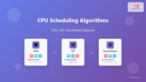
CPU Scheduling Algorithms: FCFS, SJF, Round Robin Complete Guide
CPU scheduling is a fundamental concept in operating systems that determines how processes are allocated processor time. The CPU scheduler...

Preemptive vs Non-Preemptive Scheduling: Complete Guide to CPU Scheduling in Operating Systems
Understanding CPU Scheduling in Operating Systems CPU scheduling is one of the most critical functions of an operating system, determining...

Virtual CPU Scheduling: Complete Guide to Time-sharing Physical Processors
Virtual CPU scheduling is the cornerstone of modern operating systems, enabling multiple processes to share limited physical processors efficiently. This...

Fair Share Scheduling: Resource Allocation by User Groups in Operating Systems
Introduction to Fair Share Scheduling Fair Share Scheduling (FSS) is a sophisticated CPU scheduling algorithm designed to allocate computing resources...

Priority Scheduling Algorithm: Complete Implementation Guide with Examples
What is Priority Scheduling Algorithm? Priority scheduling is a CPU scheduling algorithm where each process is assigned a priority value,...

Real-time Scheduling: Hard and Soft Real-time Systems in Operating Systems
Real-time scheduling is a critical component of operating systems that manage tasks with strict timing requirements. Unlike traditional scheduling systems...

Completely Fair Scheduler: Linux CFS Algorithm Deep Dive
The Linux Completely Fair Scheduler (CFS) revolutionized process scheduling in the Linux kernel when it was introduced in version 2.6.23....
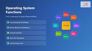
Operating System Functions: Core Components and System Responsibilities
An operating system (OS) serves as the fundamental software layer that manages computer hardware resources and provides essential services to...

Shortest Job First Scheduling: SJF Algorithm Explained with Examples and Implementation
What is Shortest Job First (SJF) Scheduling? Shortest Job First (SJF) scheduling is a CPU scheduling algorithm that selects the...
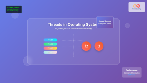
Thread in Operating System: Lightweight Processes and Multithreading Explained
What are Threads in Operating Systems? A thread is the smallest unit of execution within a process that can be...

Round Robin Scheduling: Time Quantum and Performance Analysis in Operating Systems
What is Round Robin Scheduling? Round Robin (RR) scheduling is a preemptive CPU scheduling algorithm that assigns equal time slices,...