NumPy is a cornerstone of scientific computing in Python, offering powerful array manipulation capabilities. Matplotlib, on the other hand, provides a comprehensive toolkit for creating static, animated, and interactive visualizations. This article explores the seamless integration of NumPy and Matplotlib, allowing you to visualize your NumPy arrays effectively and gain deeper insights from your data.

Basic Plotting with Matplotlib

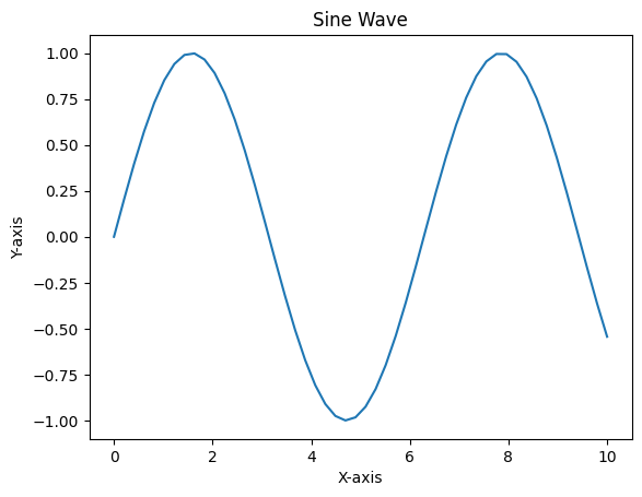
Matplotlib’s pyplot module is the foundation for creating plots. Its plot() function is a versatile tool for generating line graphs.

import numpy as np
import matplotlib.pyplot as plt

# Sample data
x = np.linspace(0, 10, 50)
y = np.sin(x)

# Creating the plot
plt.plot(x, y)

# Adding labels and title
plt.xlabel('X-axis')
plt.ylabel('Y-axis')
plt.title('Sine Wave')

# Displaying the plot
plt.show()

Output:

Explanation:

1. Importing Libraries: We start by importing the necessary libraries, NumPy and Matplotlib’s pyplot.
2. Generating Data: We create a NumPy array x representing the x-axis values using np.linspace(), which generates evenly spaced numbers over a specified interval. The y array contains the corresponding sine values of the x array.
3. Plotting: plt.plot(x, y) creates a line plot with x as the horizontal axis and y as the vertical axis.
4. Labels and Title: We enhance the plot’s clarity by adding labels to the axes (plt.xlabel() and plt.ylabel()) and a descriptive title (plt.title()).
5. Displaying: plt.show() renders the plot on the screen.

Visualizing Multidimensional Arrays

NumPy’s strength lies in its ability to work with multidimensional arrays. Matplotlib provides various methods for visualizing such arrays:

1. Image Representation with imshow()

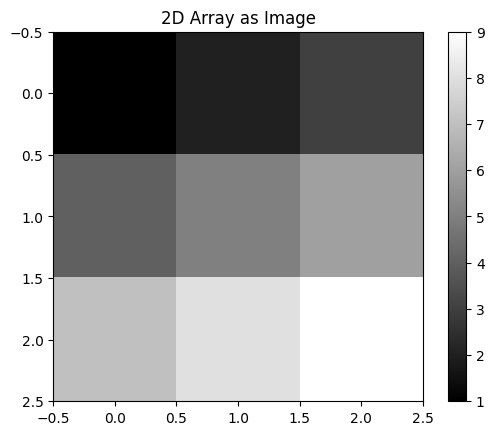
The imshow() function is designed for displaying images, which are fundamentally 2D arrays.

import numpy as np
import matplotlib.pyplot as plt

# Creating a 2D array
image_data = np.array([[1, 2, 3],
                     [4, 5, 6],
                     [7, 8, 9]])

# Displaying the array as an image
plt.imshow(image_data, cmap='gray')  # 'gray' is a colormap
plt.colorbar()  # Adding a colorbar
plt.title('2D Array as Image')
plt.show()

Output:

Explanation:

• imshow(): Takes a NumPy array and visualizes it as an image.
• cmap: Specifies the colormap to use for mapping data values to colors. Here, 'gray' creates a grayscale image.
• colorbar(): Adds a colorbar to the plot, associating color intensities with data values.

2. Surface Plots with plot_surface()

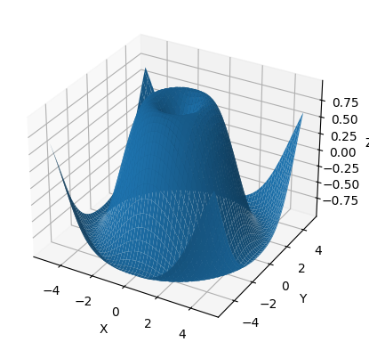
For 3D data represented as 2D arrays, Matplotlib’s plot_surface() function creates a surface plot.

from mpl_toolkits.mplot3d import Axes3D
import matplotlib.pyplot as plt
import numpy as np

# Create data for the surface plot
x = np.arange(-5, 5, 0.1)
y = np.arange(-5, 5, 0.1)
X, Y = np.meshgrid(x, y)
Z = np.sin(np.sqrt(X**2 + Y**2))

# Creating the 3D plot
fig = plt.figure()
ax = fig.add_subplot(projection='3d')
ax.plot_surface(X, Y, Z)
ax.set_xlabel('X')
ax.set_ylabel('Y')
ax.set_zlabel('Z')
plt.show()

Output:

Explanation:

• Axes3D: Imports the necessary 3D plotting capabilities.
• meshgrid(): Creates coordinate matrices for the x and y axes.
• plot_surface(): Plots the surface defined by the X, Y, and Z arrays.
• set_xlabel(), set_ylabel(), set_zlabel(): Add labels for the x, y, and z axes.

3. Contour Plots with contour()

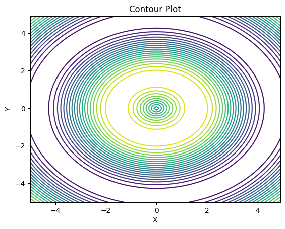
Contour plots show lines of constant value in a 2D array. They are particularly helpful for visualizing continuous data.

import matplotlib.pyplot as plt
import numpy as np

# Create data for the contour plot
x = np.arange(-5, 5, 0.1)
y = np.arange(-5, 5, 0.1)
X, Y = np.meshgrid(x, y)
Z = np.sin(np.sqrt(X**2 + Y**2))

# Creating the contour plot
plt.contour(X, Y, Z, 20)
plt.xlabel('X')
plt.ylabel('Y')
plt.title('Contour Plot')
plt.show()

Output:

Explanation:

• contour(): Creates a contour plot from the provided data. The number 20 represents the number of contour levels.

Advanced Visualization Techniques

Matplotlib offers advanced visualization capabilities for exploring and presenting complex data:

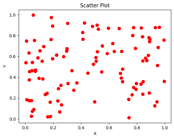
1. Scatter Plots with scatter()

Scatter plots are ideal for visualizing the relationship between two variables, particularly when the data points are discrete.

import matplotlib.pyplot as plt
import numpy as np

# Generate random data for the scatter plot
x = np.random.rand(100)
y = np.random.rand(100)

# Create the scatter plot
plt.scatter(x, y, s=50, c='red', marker='o')  # Adjust size (s), color (c), and marker
plt.xlabel('X')
plt.ylabel('Y')
plt.title('Scatter Plot')
plt.show()

Output:

Explanation:

• scatter(): Takes two arrays for x and y coordinates, allowing you to customize the size, color, and marker style of each data point.

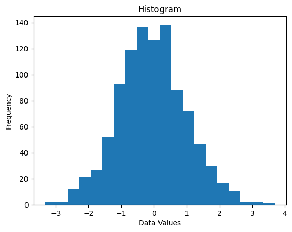
2. Histograms with hist()

Histograms visualize the frequency distribution of a dataset. They are useful for understanding data patterns and outliers.

import matplotlib.pyplot as plt
import numpy as np

# Create data for the histogram
data = np.random.randn(1000)  # Generate 1000 random numbers from a normal distribution

# Create the histogram
plt.hist(data, bins=20)  # Specify the number of bins
plt.xlabel('Data Values')
plt.ylabel('Frequency')
plt.title('Histogram')
plt.show()

Output:

Explanation:

• hist(): Generates a histogram from the provided data, dividing the data into a specified number of bins.

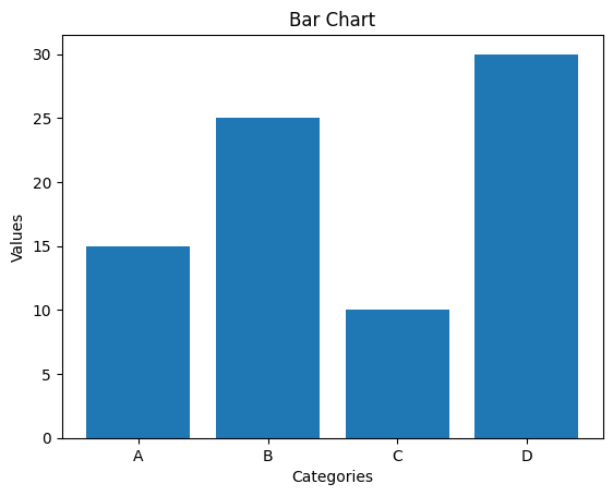
3. Bar Charts with bar()

Bar charts are effective for representing categorical data, comparing values across different groups, or showing trends over time.

import matplotlib.pyplot as plt
import numpy as np

# Data for the bar chart
categories = ['A', 'B', 'C', 'D']
values = [15, 25, 10, 30]

# Create the bar chart
plt.bar(categories, values)
plt.xlabel('Categories')
plt.ylabel('Values')
plt.title('Bar Chart')
plt.show()

Output:

Explanation:

• bar(): Creates a bar chart with the provided categories and values.

Combining NumPy and Matplotlib for Powerful Visualization

The true power of NumPy and Matplotlib lies in their synergy. NumPy enables efficient data manipulation, and Matplotlib leverages the resulting arrays to create insightful visualizations.

Example: Visualizing Image Transformations

Let’s demonstrate how NumPy and Matplotlib can work together to visualize image transformations.

import numpy as np
import matplotlib.pyplot as plt

# Load an image (replace with your image path)
image_data = plt.imread('your_image.jpg')

# Apply a transformation (e.g., rotate)
angle = 45  # Rotation angle in degrees
rotated_image = np.rot90(image_data, k=angle // 90)

# Display the original and rotated images
fig, axes = plt.subplots(1, 2, figsize=(10, 5))

axes[0].imshow(image_data)
axes[0].set_title('Original Image')

axes[1].imshow(rotated_image)
axes[1].set_title('Rotated Image')

plt.show()

Explanation:

1. Image Loading: We use plt.imread() to load an image file into a NumPy array.
2. Transformation: NumPy’s rot90() function rotates the image array by 90 degrees multiple times to achieve the desired rotation angle.
3. Visualization: We use plt.subplots() to create a figure with two subplots side by side for displaying the original and rotated images.

Key Point: This example showcases how NumPy’s array manipulation capabilities combined with Matplotlib’s visualization tools allow you to perform and visually inspect complex image transformations effortlessly.

Conclusion

NumPy and Matplotlib form a powerful combination for data visualization in Python. With NumPy’s array processing power and Matplotlib’s rich plotting features, you can gain insights from your data by creating a wide range of informative and compelling visualizations. Whether it’s analyzing images, exploring 3D datasets, or creating insightful charts, NumPy and Matplotlib provide the tools you need to bring your data to life.