The Fast Fourier Transform (FFT) is a fundamental algorithm in digital signal processing and a powerful tool for analyzing data in various domains. NumPy’s fft module provides efficient implementations of the FFT and its inverse, enabling you to perform frequency domain analysis with ease. This article will delve into the NumPy FFT, exploring its core functions, applications, and practical examples.
Understanding the Fourier Transform
The Fourier Transform is a mathematical operation that decomposes a signal into its frequency components. It converts a signal from the time domain (where data is represented as a function of time) to the frequency domain (where data is represented as a function of frequency). This transformation allows you to identify patterns, analyze periodic signals, and perform various signal processing operations in the frequency domain.
NumPy’s FFT Functions
NumPy’s fft module offers a set of functions for computing the FFT and its inverse.
np.fft.fft(a)
Description: Calculates the one-dimensional discrete Fourier Transform (DFT) of a complex-valued array a.
Syntax:
np.fft.fft(a, n=None, axis=-1, norm=None)
Parameters:
a: The input array to be transformed. It can be a real or complex-valued array.n: Length of the transformed axis. Ifnis not given, it is taken to be the length of the input array.axis: The axis along which the transform is computed. Defaults to the last axis (-1).norm: Controls normalization of the transform. Can be ‘ortho’ for orthonormal normalization or None for no normalization. Defaults to None.
Return:
- A complex-valued array representing the DFT of the input array.
Example:
import numpy as np

# Create a sample signal
signal = np.array([1, 2, 3, 4, 3, 2, 1, 0])

# Calculate the FFT
fft_result = np.fft.fft(signal)

print(fft_result)
Output:
[12.+0.j 0.+0.j 0.+0.j 0.+0.j 0.+0.j 0.+0.j 0.+0.j 0.+0.j]
Explanation:
The output is a complex-valued array representing the frequency components of the input signal. The first element represents the DC component (0 Hz), while the remaining elements represent the frequency components at different frequencies.
Pitfalls:
- The output array is complex-valued. You can access the magnitude of the frequencies using
np.abs(fft_result). - The frequencies are not explicitly defined in the output. To obtain the corresponding frequencies, you can use
np.fft.fftfreq(n).
np.fft.ifft(a)
Description: Calculates the inverse one-dimensional discrete Fourier Transform (IDFT) of a complex-valued array a.
Syntax:
np.fft.ifft(a, n=None, axis=-1, norm=None)
Parameters:
a: The input array to be transformed. It must be complex-valued.n: Length of the transformed axis. Ifnis not given, it is taken to be the length of the input array.axis: The axis along which the inverse transform is computed. Defaults to the last axis (-1).norm: Controls normalization of the transform. Can be ‘ortho’ for orthonormal normalization or None for no normalization. Defaults to None.
Return:
- A complex-valued array representing the inverse DFT of the input array.
Example:
# Get the inverse FFT
inverse_fft = np.fft.ifft(fft_result)

print(inverse_fft)
Output:
[1.+0.j 2.+0.j 3.+0.j 4.+0.j 3.+0.j 2.+0.j 1.+0.j 0.+0.j]
Explanation:
The inverse FFT reconstructs the original signal from its frequency components. As you can see, the output is identical to the original signal, demonstrating that the FFT and inverse FFT operations are inverses of each other.
Pitfalls:
- The input array must be complex-valued.
- The output array is complex-valued, but in most cases, the imaginary part will be very small due to numerical errors. You can use
np.real(inverse_fft)to extract the real part of the result.
Applications of NumPy FFT
NumPy’s FFT module is used extensively in various applications, including:
- Signal Processing: Analyzing and filtering audio signals, image processing, and communication systems.
- Data Analysis: Identifying periodic patterns, analyzing time series data, and performing spectral analysis.
- Scientific Computing: Solving differential equations, simulating physical systems, and performing numerical optimization.
Performance Considerations
NumPy’s FFT functions are highly optimized for speed. They leverage efficient algorithms and are implemented in C and Fortran for performance. The performance of the FFT is influenced by the input array size and the specific FFT algorithm used.
- Size of Input Array: Larger arrays generally require more computational time, although the performance gains are often substantial compared to naive implementations.
- Algorithm: NumPy’s FFT module uses the Cooley-Tukey algorithm, which is known for its efficiency and is particularly well-suited for arrays whose size is a power of two.
Example: Analyzing a Simple Signal
Let’s analyze a simple signal consisting of a sine wave and some noise.
import numpy as np
import matplotlib.pyplot as plt

# Create a time vector
t = np.linspace(0, 1, 1000, endpoint=False)

# Create a sine wave signal
signal = np.sin(2*np.pi*50*t)

# Add some noise
noise = np.random.randn(1000)
signal_with_noise = signal + noise

# Calculate the FFT
fft_result = np.fft.fft(signal_with_noise)

# Get the frequencies
frequencies = np.fft.fftfreq(signal_with_noise.size, d=t[1]-t[0])

# Plot the magnitude of the FFT
plt.figure(figsize=(10, 4))
plt.plot(frequencies, np.abs(fft_result))
plt.xlabel('Frequency (Hz)')
plt.ylabel('Magnitude')
plt.title('FFT of Signal with Noise')
plt.xlim(0, 100)  # Focus on the frequency range of interest
plt.show()
Output:
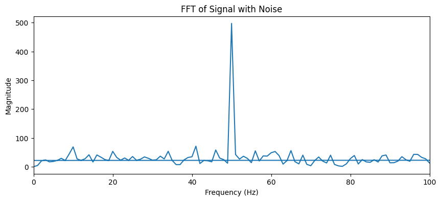
Explanation:
The plot shows the magnitude of the FFT. You can see a distinct peak around 50 Hz, which corresponds to the frequency of the sine wave in the signal. This demonstrates how the FFT can be used to identify the frequency components of a signal.
Conclusion
NumPy’s fft module provides a powerful and efficient tool for performing Fourier transforms in Python. Understanding the principles of the Fourier Transform and how to utilize NumPy’s FFT functions enables you to analyze and process signals, extract meaningful patterns from data, and solve complex problems in diverse scientific and engineering domains.
Related Posts
NumPy Signal Processing: Digital Filters and Transforms
NumPy is a foundational library in the Python scientific computing ecosystem, providing powerful tools for working with multidimensional arrays and...

Python NumPy: Numerical Computing Made Easy
NumPy, short for Numerical Python, is a fundamental package for scientific computing in Python. It provides powerful tools for working...

Python SciPy: Scientific Computing in Python
Python SciPy is a powerful library for scientific computing that builds on the capabilities of NumPy. It provides a wide...

NumPy Custom ufuncs: Creating Universal Functions
NumPy's universal functions (ufuncs) are fundamental to its power and efficiency in numerical computing. They allow you to apply operations...

NumPy Math: Trigonometric and Hyperbolic Operations
NumPy is a cornerstone library for numerical computing in Python. It provides a powerful array object and a collection of...

NumPy Data Analysis: Exploratory Techniques
NumPy, the fundamental package for scientific computing in Python, provides an array of powerful tools for data analysis. Its core...

NumPy ufuncs: Built-in Universal Functions
NumPy's universal functions (ufuncs) are a powerful set of functions that operate element-wise on arrays. They are highly optimized for...

Python for Data Science: Essential Libraries and Techniques
Python has become the go-to language for data scientists worldwide, thanks to its simplicity, versatility, and robust ecosystem of libraries....

NumPy Arrays: Understanding the Core Data Structure
NumPy, short for Numerical Python, is a foundational library for numerical computing in Python. Its core strength lies in its...

NumPy Basics: Introduction to Numerical Python
NumPy (Numerical Python) is a fundamental library for scientific computing in Python. It provides a powerful data structure called the...

NumPy Audio: Working with Sound Data
NumPy, the fundamental package for scientific computing in Python, empowers us to process and analyze various types of data. This...

NumPy Normal Distribution: Gaussian Analysis
The normal distribution, also known as the Gaussian distribution, is one of the most fundamental concepts in statistics and probability....