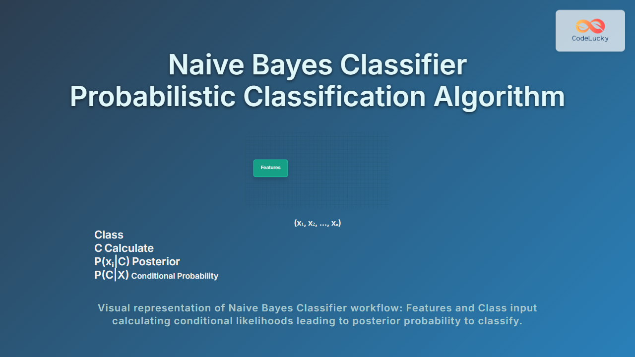
The Naive Bayes Classifier is a simple yet effective probabilistic classification algorithm rooted in Bayes’ theorem. It leverages conditional probability to assign class labels to data points based on their features, assuming feature independence. This article presents an in-depth explanation of Naive Bayes, its working principles, types, mathematical background, and practical examples with clear visualizations to help grasp its utility in machine learning and data science applications.
What is the Naive Bayes Classifier?
Naive Bayes is a probabilistic classification algorithm that predicts the category of a given data point by calculating the posterior probability of each class using Bayes’ theorem. It is called “naive” due to the simplifying assumption that all features contribute independently to the outcome, which rarely holds in real data but works surprisingly well in practice.
Bayes’ Theorem: The Core Principle
At the heart of the Naive Bayes classifier lies Bayes’ Theorem, which relates the conditional and marginal probabilities of random events:
P(C|X) = (P(X|C) * P(C)) / P(X)
P(C|X)is the posterior probability of classCgiven feature vectorX.P(X|C)is the likelihood of feature vectorXgiven classC.P(C)is the prior probability of classC.P(X)is the evidence or total probability ofX.
The classifier predicts the class C that maximizes P(C|X).
Naive Bayes Assumption: Feature Independence
The classifier simplifies calculations by assuming that the features are conditionally independent given the class:
P(X|C) = P(x₁, x₂, ..., xₙ | C) = P(x₁|C) × P(x₂|C) × ... × P(xₙ|C)
This allows the model to easily compute the likelihood of the features collectively by multiplying their individual probabilities.
Types of Naive Bayes Classifiers
Several Naive Bayes variants exist based on the nature of the data features:
- Gaussian Naive Bayes: For continuous numerical features assumed to follow a normal distribution.
- Multinomial Naive Bayes: Suitable for discrete features like word counts in text classification.
- Bernoulli Naive Bayes: Designed for binary/boolean features presence or absence.
Step-by-Step Example: Classifying Emails as Spam or Not Spam
Consider a simplified problem where we want to classify emails into Spam or Not Spam based on the presence of the words “win” and “money.” Let’s calculate the probability an email is spam given these features.
| Class | P(Class) | P(“win” | Class) | P(“money” | Class) |
|---|---|---|---|
| Spam | 0.4 | 0.7 | 0.8 |
| Not Spam | 0.6 | 0.1 | 0.3 |
For an email that contains both words “win” and “money,” calculate posterior probabilities:
P(Spam | win, money) ∝ P(win | Spam) * P(money | Spam) * P(Spam)
= 0.7 * 0.8 * 0.4 = 0.224

P(Not Spam | win, money) ∝ P(win | Not Spam) * P(money | Not Spam) * P(Not Spam)
= 0.1 * 0.3 * 0.6 = 0.018
Since 0.224 > 0.018, the email is classified as Spam.
Advantages of Naive Bayes
- Fast and Efficient: Requires a small amount of training data to estimate parameters.
- Handles High Dimensional Data: Performs well in text classification and document categorization.
- Simple to Implement: Easy to understand with a solid probabilistic foundation.
Limitations of Naive Bayes
- Feature Independence Assumption: Often unrealistic; correlated features can reduce accuracy.
- Zero Probability Problem: If a class-feature combination never appears in training, probability estimates become zero (can be solved with smoothing).
- Not Ideal for Complex Relationships: Struggles with datasets where interactions between features are crucial.
Interactive Code Example (Python)
Below is a simple Python snippet demonstrating Gaussian Naive Bayes classification using the scikit-learn library:
from sklearn.datasets import load_iris
from sklearn.model_selection import train_test_split
from sklearn.naive_bayes import GaussianNB
from sklearn.metrics import accuracy_score

# Load Iris dataset
iris = load_iris()
X, y = iris.data, iris.target

# Split dataset into train and test sets
X_train, X_test, y_train, y_test = train_test_split(X, y, test_size=0.3, random_state=42)

# Initialize Gaussian Naive Bayes classifier
gnb = GaussianNB()

# Train the model
gnb.fit(X_train, y_train)

# Predict on test set
y_pred = gnb.predict(X_test)

# Calculate accuracy
print('Accuracy:', accuracy_score(y_test, y_pred))
Summary
The Naive Bayes Classifier is a cornerstone of probabilistic machine learning, known for its simplicity and surprising effectiveness in many real-world classification problems like spam detection, sentiment analysis, and document classification. Understanding its assumptions and applying the right variant depending on data type can lead to robust, explainable models. This article aimed to provide a clear, detailed guide supported by mathematical foundations and practical examples for a comprehensive grasp of Naive Bayes.
