Logistic Regression is a fundamental binary classification algorithm widely used in machine learning and statistics for predicting categorical outcomes. It models the probability that a given input belongs to a particular class using the logistic function, making it ideal for classification problems with two possible labels, such as spam detection, disease diagnosis, or customer churn prediction.
Understanding Logistic Regression
Unlike linear regression, which predicts continuous values, logistic regression estimates probabilities bounded between 0 and 1 using the sigmoid or logistic function. The core equation for logistic regression is:
hθ(x) = 1 / (1 + e-z), where z = θ0 + θ1x1 + θ2x2 + ... + θnxnThe hypothesis function hθ(x) outputs the probability that the dependent variable belongs to class 1 given input features x, weighted by parameters θ.
Key Components of Logistic Regression
- Features (x): Independent variables or predictors.
- Parameters (θ): Weights learned by the model during training.
- Sigmoid function: Converts linear output to probability.
- Cost function: Log-loss or cross-entropy used for optimization.
- Decision boundary: Threshold (usually 0.5) to classify output.
Cost Function and Model Training
Logistic regression uses the log-likelihood cost function (often called cross-entropy loss) to measure how well the predicted probabilities match the actual classes:
J(θ) = - (1/m) ∑ [y log(hθ(x)) + (1 - y) log(1 - hθ(x))]Where:
m= number of training examplesy= true class label (0 or 1)hθ(x)= predicted probability
The model parameters θ are optimized to minimize this cost function using methods like Gradient Descent.
Logistic Regression Algorithm Steps
Binary Classification Example
Consider a simple dataset with one feature x (e.g., exam scores) and a binary target y (pass=1, fail=0). The logistic regression model can predict the probability of passing:
| Exam Score (x) | Pass (y) |
|---|---|
| 54 | 0 |
| 67 | 0 |
| 72 | 1 |
| 88 | 1 |
| 93 | 1 |
Using logistic regression, after training, the model could output probabilities like 0.23, 0.46, 0.7, 0.9, and 0.95 respectively for these points. Applying a threshold of 0.5, scores above 0.5 predict passing, below predict failing.
Visualizing the Logistic Curve
The logistic function forms an S-shaped curve that smoothly maps scores to probabilities:

Higher scores correspond to higher passing probabilities approaching 1, and lower scores approach 0.
Interactive Logistic Regression Concept (Example)
Probability Calculator: Enter a score to get passing probability.
Advantages of Logistic Regression
- Interpretability: Coefficients show feature impact.
- Computationally efficient and fast.
- Produces calibrated probabilities for classification.
- Widely used baseline algorithm for binary classification.
Limitations
- Assumes linear decision boundary in feature space.
- Not ideal for complex relationships or multi-class directly without extensions.
- Sensitive to outliers and multicollinearity.
Summary
Logistic regression remains a primary binary classification technique in machine learning due to its simplicity, effectiveness, and interpretability. By leveraging the logistic function to map inputs to probabilities, it allows decision-making on binary outcomes with intuitive mathematical foundation. Understanding logistic regression helps build a foundation for more complex classification methods.