Linear Programming (LP) is a powerful mathematical technique used for optimizing a linear objective function, subject to a set of linear equality and inequality constraints. Among the various methods to solve LP problems, the Simplex Method stands out as one of the most influential and widely applied optimization algorithms in fields such as operations research, economics, engineering, and computer science.
This article presents an in-depth, SEO-friendly exploration of the Simplex Method with clear conceptual explanations, step-by-step examples, and visualizations to facilitate understanding, especially for those new to optimization algorithms.
What Is Linear Programming?
Linear Programming involves optimizing a linear function of variables, called the objective function, while satisfying a set of linear constraints. These constraints restrict the possible values the variables can take, defining a region called the feasible region. The goal is to find the point in this region that maximizes or minimizes the objective function.
- Objective function example:
Maximize z = 3x + 5y - Constraints example:
2x + y ≤ 144x + 3y ≤ 35x ≥ 0, y ≥ 0
Understanding the Simplex Method
The Simplex Method is an iterative algorithm that navigates the vertices of the feasible region (a convex polytope) to locate the optimal solution. Since a linear function’s optimum over a convex polygon occurs at one of its vertices, the Simplex Method moves from vertex to vertex, improving the objective value at each step until it reaches the maximum or minimum possible.
The key advantage is efficiency: the Simplex method often solves problems much faster than evaluating all possible feasible points, especially in high-dimensional spaces.
Step-by-Step Outline of the Simplex Method
- Convert all constraints into equalities by adding slack variables.
- Set up the initial Simplex tableau with variables, coefficients, and constants.
- Identify the entering variable (most negative coefficient in the objective row for maximization).
- Calculate the leaving variable using the minimum ratio test.
- Perform pivot operations to update the tableau.
- Repeat the process until there are no negative coefficients in the objective function row.
- Read off the solution from the final tableau.
Example: Maximizing Profit Using Simplex Method
Consider a factory producing two products, Product A and Product B. The goal is to maximize profit given resource constraints.
- Profit per unit: Product A = $40, Product B = $30
- Resource constraints:
- Material: 3 units for A, 2 units for B; total available = 18 units
- Labor: 4 hours for A, 3 hours for B; total available = 24 hours
- Non-negativity constraints: \(x, y \geq 0\)
Formulate the problem:
Maximize \( z = 40x + 30y \)
Subject to:
3x + 2y ≤ 18
4x + 3y ≤ 24
x, y ≥ 0
Convert constraints to equalities by adding slack variables \(s_1\) and \(s_2\):
3x + 2y + s₁ = 18
4x + 3y + s₂ = 24
s₁, s₂ ≥ 0
Initial Simplex Tableau
| Basis | x | y | s₁ | s₂ | RHS |
|---|---|---|---|---|---|
| s₁ | 3 | 2 | 1 | 0 | 18 |
| s₂ | 4 | 3 | 0 | 1 | 24 |
| z | -40 | -30 | 0 | 0 | 0 |
Simplex Iterations (Summary)
- Step 1: Enter variable \(x\) (most negative coefficient in \(z\) row: -40).
- Step 2: Determine leaving variable by minimum ratio test:
- For s₁: 18 / 3 = 6
- For s₂: 24 / 4 = 6
Minimum ratio is 6; choose either (e.g., s₁).
- Step 3: Pivot around the element in s₁ row and x column.
- Step 4: Update tableau and repeat until no negative coefficients in the profit row remain.
The final solution gives \(x = 6\), \(y = 0\), maximum profit \(z = 240\).
Visualizing the Feasible Region and Optimal Point
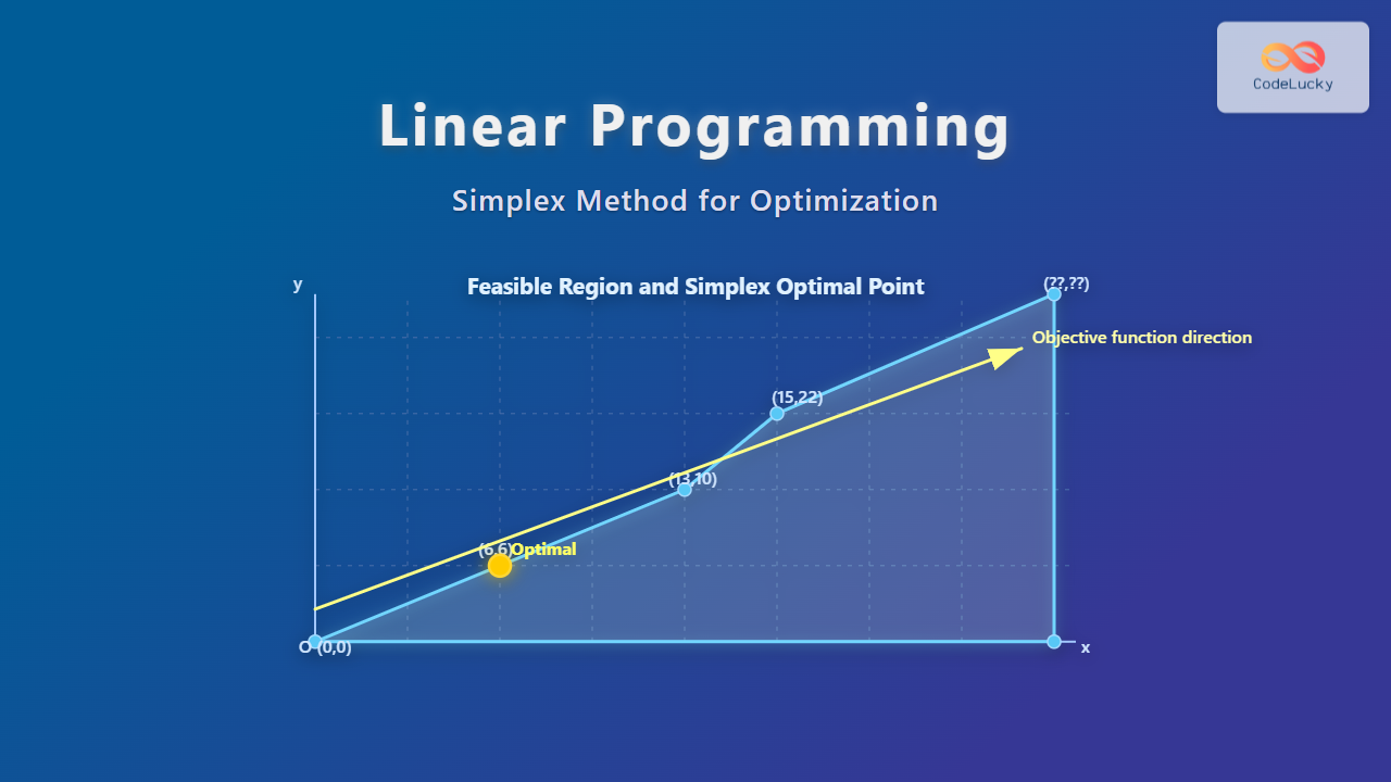
The feasible region described by the inequalities can be represented graphically, where the shaded polygon is the feasible set. The Simplex method progresses along the edges and vertices of this polygon, evaluating the objective function, until it reaches the optimal vertex.
Interactive Consideration
An interactive LP solver or visualization tool could allow users to adjust constraints and coefficients dynamically, witnessing the Simplex Method’s movement and outcome changes in real-time. Such tools help deepen understanding by illustrating the algorithm’s geometric intuition.
Summary & SEO Keywords
The Simplex Method efficiently solves linear programming problems by iteratively moving along the vertices of the feasible region to find the optimal value of a linear objective function. Understanding the method requires grasping iteration, tableau formation, pivot operations, and the geometric interpretation of LP problems. This article has demonstrated detailed example applications, visual diagrams, and a step-by-step approach to mastering the Simplex algorithm.
Key SEO terms: Linear Programming, Simplex Method, Optimization Algorithm, Operations Research, LP Example, Feasible Region, Slack Variables, Optimal Solution.

