0/1 Knapsack Problem: Dynamic Programming Solution Explained with Examples

The 0/1 Knapsack Problem is one of the most famous and foundational problems in computer science and optimization. It is widely used to teach dynamic programming, a problem-solving method where complex problems are broken down into simpler subproblems. In this article, we will explore the 0/1 Knapsack problem in depth, explain how to solve it using dynamic programming, provide visualizations, and implement it in Python with practical examples.

What is the 0/1 Knapsack Problem?

The problem can be stated as follows:

You are given a set of items, each with a weight and a value. You need to choose a subset of items to put into a knapsack of fixed capacity. The goal is to maximize the total value without exceeding the capacity of the knapsack. Each item can either be included or excluded (hence the name 0/1).

Problem Definition

• Input: list of items with weights and values, and maximum capacity W.
• Decision: include or exclude each item.
• Goal: maximize total value without exceeding capacity.

Understanding with a Real-life Example

Imagine you are going camping and your backpack can hold only 10kg. You have items like food, water, tent, flashlight, and clothes, each with a certain weight and value. You must decide which combination to pack to maximize the usefulness (value) of your trip, without overloading your backpack.

Brute Force Solution (Inefficient)

The brute force approach tries all possible combinations of items. For n items, there are 2ⁿ possibilities. This becomes impractical as the number of items grows. Hence, we need Dynamic Programming for efficiency.

Dynamic Programming Solution

The 0/1 Knapsack problem exhibits two properties that make it suitable for dynamic programming:

• Overlapping Subproblems: The same subproblem (choosing items with smaller capacity) gets solved multiple times.
• Optimal Substructure: The optimal solution of the whole problem depends on the optimal solutions of subproblems.

Recursive Relation

If we have n items and a capacity W, the maximum value can be defined as:

knapsack(n, W) = max(
    value[n-1] + knapsack(n-1, W - weight[n-1]),  // including item n-1
    knapsack(n-1, W)                              // excluding item n-1
)

Dynamic Programming Table Approach

We use a 2D DP table where:

• dp[i][w] = maximum value achievable with first i items and knapsack capacity w.

Step-by-Step Example

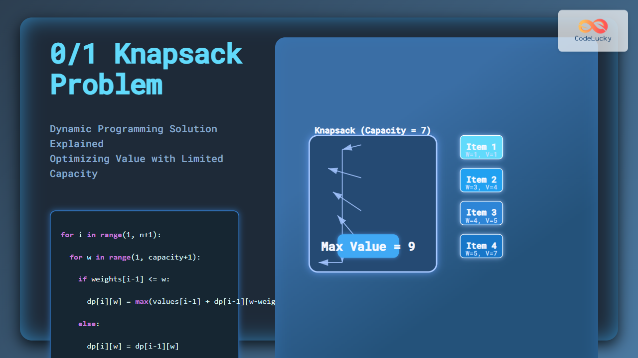
Consider the following items with capacity W=7:

Item	Weight	Value
1	1	1
2	3	4
3	4	5
4	5	7

We construct the DP table (dp[i][w]):

   Capacity (W) →  0  1  2  3  4  5  6  7
Items
0                0  0  0  0  0  0  0  0
1 (w=1,v=1)      0  1  1  1  1  1  1  1
2 (w=3,v=4)      0  1  1  4  5  5  5  5
3 (w=4,v=5)      0  1  1  4  5  6  6  9
4 (w=5,v=7)      0  1  1  4  5  7  8  9

The maximum achievable value for capacity 7 is 9.

Python Implementation

def knapsack(weights, values, capacity):
    n = len(values)
    dp = [[0 for _ in range(capacity + 1)] for _ in range(n + 1)]

    for i in range(1, n + 1):
        for w in range(1, capacity + 1):
            if weights[i-1] <= w:
                dp[i][w] = max(values[i-1] + dp[i-1][w-weights[i-1]], dp[i-1][w])
            else:
                dp[i][w] = dp[i-1][w]

    return dp[n][capacity]

# Example usage
weights = [1, 3, 4, 5]
values = [1, 4, 5, 7]
capacity = 7
print("Maximum Value:", knapsack(weights, values, capacity))

Output

Maximum Value: 9

Time and Space Complexity

• Time Complexity: O(n * W) where n = number of items, W = capacity.
• Space Complexity: O(n * W) for DP table. Can be optimized to O(W) using a 1D array.

Optimized DP Implementation with 1D Array

def knapsack_optimized(weights, values, capacity):
    n = len(values)
    dp = [0] * (capacity + 1)

    for i in range(n):
        for w in range(capacity, weights[i]-1, -1):
            dp[w] = max(dp[w], values[i] + dp[w - weights[i]])

    return dp[capacity]

# Example usage
print("Maximum Value (Optimized):", knapsack_optimized(weights, values, capacity))

Interactive Idea

You can make the 0/1 Knapsack problem interactive using sliders for weight, value, and capacity in a web-based visualization. This allows users to dynamically adjust inputs and see how the optimal selection changes.

Applications of 0/1 Knapsack Problem

• Resource allocation in real-time systems.
• Budget management in project planning.
• Cryptography and subset sum based problems.
• Load balancing and cloud computing.

Conclusion

The 0/1 Knapsack Problem demonstrates the power of dynamic programming in solving optimization problems that would otherwise be infeasible by brute force. Mastering this concept builds the foundation for tackling more complex problems in algorithms, computer science, and operations research. By visualizing the DP table and implementing Python solutions, you now have a comprehensive understanding of solving the knapsack problem effectively.