Jump Search Algorithm: Square Root Searching Technique Explained with Examples

Searching efficiently within sorted data is a crucial problem in computer science. While linear search checks elements one by one and binary search halves the search interval recursively, the Jump Search Algorithm offers a middle-ground by making fixed-size jumps, reducing the number of comparisons. This algorithm uses the square root searching technique, balancing efficiency with simplicity.

Table of Contents

What is Jump Search Algorithm?

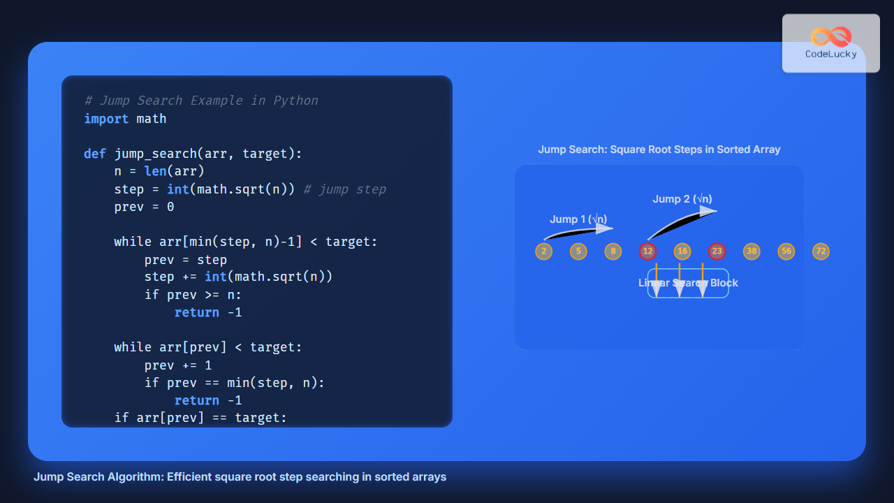
Jump Search is a searching technique designed for sorted arrays. Instead of checking every element sequentially, it skips ahead by a block of size √n (where n is the array length). Once it overshoots or finds a block likely containing the target, it performs a linear search inside that block.

When to Use Jump Search?

Works only on sorted arrays.
Faster than linear search for large datasets.
Preferable when binary search is harder to implement (e.g., linked structures with sequential access).

How Jump Search Works

Choose a jump step = √n.
Start from the first element and jump ahead by step until the current element exceeds the target or the array end is reached.
Perform a linear search backward within the block where the target might exist.
If found, return its index; otherwise, return -1.

Example Walkthrough

Suppose we have a sorted array:

arr = [2, 5, 8, 12, 16, 23, 38, 56, 72, 91]
target = 23
n = 10
step = √n ≈ 3

Steps:

Check arr[0] = 2, jump to arr[3] = 12.
Check arr[3] = 12, jump to arr[6] = 38.
23 < 38 → linear search back in block [12, 16, 23].
Found 23 at index 5.

Python Implementation of Jump Search


import math

def jump_search(arr, target):
    n = len(arr)
    step = int(math.sqrt(n))  # optimal step
    prev = 0

    # Jump until overshoot or target block found
    while arr[min(step, n)-1] < target:
        prev = step
        step += int(math.sqrt(n))
        if prev >= n:
            return -1

    # Linear search in identified block
    while arr[prev] < target:
        prev += 1
        if prev == min(step, n):
            return -1
    if arr[prev] == target:
        return prev
    return -1

# Example usage
arr = [2, 5, 8, 12, 16, 23, 38, 56, 72, 91]
target = 23
result = jump_search(arr, target)
print(f"Element found at index: {result}")

Output:


Element found at index: 5

Complexity Analysis

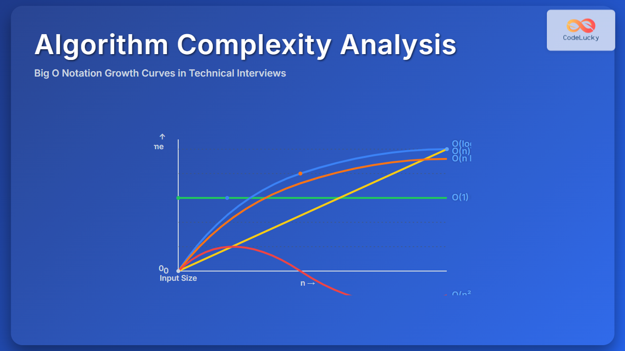
Best Case: O(1) (if the first element matches)
Average Case: O(√n)
Worst Case: O(√n) (linear scan within one block)
Space Complexity: O(1) (constant extra space)

Advantages of Jump Search

Faster than linear search for large sorted datasets.
Simpler to implement in certain sequential access structures compared to binary search.
Predictable step size makes it efficient for indexed data.

Limitations

Requires sorted input data.
Not as fast as binary search (O(log n)).
Best suited for arrays with random access; less efficient for linked lists due to jump cost.

Interactive Concept Visualization

Imagine standing on a number line. Instead of walking step by step like linear search, Jump Search makes leaps of √n steps. If you overshoot the target zone, you walk backward step by step until you find the exact number.

Conclusion

The Jump Search Algorithm provides a fine balance between simplicity and efficiency when working with sorted arrays. With a complexity of O(√n), it is significantly faster than linear search while being easier to implement than binary search in some scenarios. For practical programming, especially in cases where random access is expensive, Jump Search offers a valuable tradeoff.