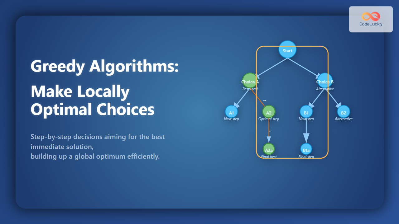
Greedy Algorithms: Make Locally Optimal Choices Explained with Examples

Greedy Algorithms are a class of optimization techniques in computer science where the strategy is simple yet powerful: at every step, make the choice that looks best at that moment (locally optimal choice). The hope is that a sequence of such decisions will lead to a globally optimal solution. While greedy algorithms do not always guarantee correctness for all problems, they excel in many classic scenarios such as job scheduling, graph algorithms, and compression techniques.

Table of Contents

Key Characteristics of Greedy Algorithms

Local Decisions: Solve problems step by step, always choosing the current best option.
No Backtracking: Once a choice is made, it is never reconsidered.
Greedy Choice Property: A global optimum can be reached by choosing local optimums.
Optimal Substructure: The problem can be broken down into subproblems that are optimal as well.

Greedy Algorithm Framework

A general structure of a greedy algorithm involves:

Sorting or selecting based on an evaluation metric (e.g., profit, weight, frequency).
Iteratively picking the best available choice.
Continuing until no more choices remain or constraints are met.

Example 1: Coin Change Problem (Greedy Approach)

Suppose you need to make a change for 93 using coins of denominations: {1, 2, 5, 10, 20, 50}. A greedy strategy is to always pick the largest coin less than or equal to the remaining amount:


def greedy_coin_change(coins, amount):
    result = []
    coins.sort(reverse=True)
    for coin in coins:
        while amount >= coin:
            amount -= coin
            result.append(coin)
    return result

print(greedy_coin_change([1,2,5,10,20,50], 93))

Output:

[50, 20, 20, 2, 1]

Here, the greedy algorithm gives the optimal answer (though for other coin systems it might fail). Visualization:

Example 2: Activity Selection Problem

Given a set of activities with start and finish times, the task is to select the maximum number of activities that don’t overlap. The greedy choice is to always pick the activity with the earliest finishing time.


activities = [(1,3), (2,4), (0,6), (5,7), (8,9), (5,9)]

def activity_selection(activities):
    activities.sort(key=lambda x: x[1])  # sort by finish time
    selected = [activities[0]]
    last_end = activities[0][1]
    for start, end in activities[1:]:
        if start >= last_end:
            selected.append((start, end))
            last_end = end
    return selected

print(activity_selection(activities))

Output:

[(1, 3), (5, 7), (8, 9)]

The selected non-overlapping activities are (1,3), (5,7), and (8,9).

Example 3: Huffman Coding (Data Compression)

Huffman Coding is a greedy algorithm used for lossless data compression. It works by building a binary tree with the smallest frequency characters near the root, ensuring more frequent symbols have shorter codes.


import heapq

def huffman_coding(freq):
    heap = [[weight, [symbol, ""]] for symbol, weight in freq.items()]
    heapq.heapify(heap)
    while len(heap) > 1:
        lo = heapq.heappop(heap)
        hi = heapq.heappop(heap)
        for pair in lo[1:]:
            pair[1] = '0' + pair[1]
        for pair in hi[1:]:
            pair[1] = '1' + pair[1]
        heapq.heappush(heap, [lo[0] + hi[0]] + lo[1:] + hi[1:])
    return sorted(heapq.heappop(heap)[1:], key=lambda p: (len(p[-1]), p))

freq = {'a':45, 'b':13, 'c':12, 'd':16, 'e':9, 'f':5}
print(huffman_coding(freq))

Sample Output:

[('a', '0'), ('b', '101'), ('c', '100'), ('d', '111'), ('e', '1101'), ('f', '1100')]

Notice how the most frequent character 'a' gets the shortest code.

Applications of Greedy Algorithms

Graph Algorithms: Prim’s and Kruskal’s algorithms for Minimum Spanning Tree, Dijkstra’s algorithm (with non-negative weights).
Scheduling and Resource Allocation: Activity selection, job scheduling, CPU task assignments.
Compression: Huffman coding, file storage optimizations.
Mathematics and Number Theory: Egyptian fraction decomposition, interval covering problems.

Advantages and Limitations

Advantages:

Simple and easy to implement.
Usually more efficient (lower complexity) compared to dynamic programming.

Limitations:

Does not always guarantee an optimal solution for all problems.
Requires careful analysis to confirm correctness before applying.

Conclusion

Greedy algorithms embody the principle of making the best local decision in hopes of achieving a global optimum. They are not universally applicable but provide elegant and highly efficient solutions for many real-world challenges—whether it’s scheduling tasks, compressing data, or finding shortest connections in graphs. A good computer scientist must learn to identify when a problem exhibits greedy properties and when more sophisticated approaches like dynamic programming are required.