Fast Fourier Transform: Comprehensive Guide to Signal Processing Algorithm

The Fast Fourier Transform (FFT) is a fundamental algorithm in signal processing and digital computation, revolutionizing how we analyze frequencies in signals efficiently. By enabling the rapid computation of the Discrete Fourier Transform (DFT), FFT underpins applications ranging from audio processing to image analysis, telecommunications, and scientific computing.

This article dives deep into the FFT algorithm, its steps, mathematical principles, example usage, and how it accelerates signal analysis with clarity and interactivity in mind—perfect for enthusiasts, students, and professionals aiming to master signal processing techniques.

What is the Fast Fourier Transform (FFT)?

The Fast Fourier Transform is an efficient algorithm to compute the Discrete Fourier Transform (DFT) and its inverse. While DFT directly analyzes a finite sequence of data points to reveal frequency components, its naive computation cost is O(N²). FFT reduces this complexity to O(N log N) where N is the number of data points, making it suitable for real-time and large-scale applications.

The key idea of FFT is to recursively break down the DFT of a sequence into smaller DFTs of its even- and odd-indexed elements, leveraging symmetries and periodicities of complex exponentials.

Mathematical Foundation of FFT

The DFT of a sequence x of length N is defined as:

 
X[k] = ∑_{n=0}^{N-1} x[n] * e^{-i 2π k n / N} ,  k = 0, 1, ..., N-1

Direct computation requires N sums of N terms each, resulting in O(N²) complexity. The FFT algorithm exploits the divide-and-conquer approach to reduce this:

Steps of the Cooley-Tukey FFT Algorithm

• Divide: Split the input sequence into even- and odd-indexed elements.
• Conquer: Recursively compute FFT on these smaller sequences.
• Combine: Merge the results using twiddle factors W_N^k = e^{-i2πk/N} for k in range 0 to N/2 – 1.

This reduces the repetitive calculations by reusing half DFT results and significantly increases computational speed.

Example: FFT on a Simple Signal

Consider a sample signal with 8 data points:

signal = [1, 0, 1, 0, 1, 0, 1, 0]

Applying FFT will quickly produce the frequency components:

import numpy as np
from matplotlib import pyplot as plt

signal = [1,0,1,0,1,0,1,0]
fft_result = np.fft.fft(signal)

plt.subplot(2,1,1)
plt.stem(signal)
plt.title("Original Signal (Time Domain)")

plt.subplot(2,1,2)
plt.stem(np.abs(fft_result))
plt.title("FFT Magnitude Spectrum (Frequency Domain)")
plt.show()

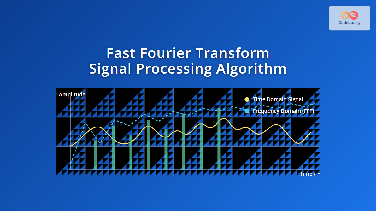
The time-domain signal shows a repeating pulse, while the magnitude FFT output reveals the spectral peaks corresponding to the periodic components of the signal.

Visualizing FFT Process

Here’s a mermaid flowchart outlining the FFT recursion and results merging:

Applications of FFT

• Audio Processing: Spectrum analysis, filtering, sound synthesis.
• Image Processing: Frequency domain filtering, image compression.
• Communications: Modulation, demodulation, signal spectrum estimation.
• Scientific Computing: Solving partial differential equations, spectral methods.

Interactive FFT Demonstration

Below is a simple interactive JavaScript example to visualize FFT on a custom signal (embedded in an HTML page) using an FFT library such as fft.js. This enables experimenting with signal values and observing frequency output live.

<input id="inputSignal" type="text" value="1,0,1,0,1,0,1,0">
<button onclick="computeFFT()">Compute FFT</button>
<pre id="outputFFT"></pre>

<script>
function computeFFT() {
  let input = document.getElementById('inputSignal').value.split(',').map(Number);
  if (input.length && (input.length & (input.length - 1)) === 0) {
    // Length must be power of 2 for classic Cooley-Tukey FFT
    let fft = new FFT(input.length);
    let complexArray = fft.createComplexArray();
    fft.realTransform(complexArray, input);
    fft.completeSpectrum(complexArray);
    let result = [];
    for(let i=0; i < complexArray.length; i += 2){
      let mag = Math.sqrt(complexArray[i]*complexArray[i] + complexArray[i+1]*complexArray[i+1]);
      result.push(mag.toFixed(2));
    }
    document.getElementById('outputFFT').textContent = result.join(', ');
  } else {
    alert("Input length must be a power of 2");
  }
}
</script>
  

Optimizations and Variants

Several FFT algorithm variants exist to optimize specific scenarios:

• Radix-2 FFT: Most common, input length is a power of 2.
• Radix-4 FFT: Operates on powers of 4, more efficient in some cases.
• Mixed-Radix FFT: Handles composite lengths by combining radix-2 and radix-3.
• Real FFT: Optimized for real-valued input signals to save computation.

Summary

The Fast Fourier Transform stands as a cornerstone algorithm for digital signal processing, turning complex frequency analysis from a computational bottleneck into an accessible, real-time tool. Mastery of FFT enhances understanding of diverse fields like audio engineering, telecommunications, and image processing.

By leveraging its recursive divide-and-conquer foundation and visualizing its recursive split-combine process, learners can grasp FFT’s power intuitively.

Experiment with code examples and interactive demonstrations to consolidate this essential algorithm knowledge and unlock new signal analysis capabilities.