Fast Fourier Transform: Efficient Polynomial Multiplication Explained

The Fast Fourier Transform (FFT) is a powerful algorithm that revolutionizes polynomial multiplication, reducing the complexity from naive quadratic time to nearly linear time. This article will deeply explore how FFT enables efficient polynomial multiplication, covering foundational concepts, algorithmic steps, and practical examples enhanced with visual explanations and clear illustrations using <div class="mermaid"> diagrams. By the end, readers will have a comprehensive understanding of FFT’s role in computational mathematics and computer science.

Understanding Polynomial Multiplication and Its Complexity

Polynomial multiplication involves multiplying two polynomials, for example, P(x) = a_0 + a_1x + a_2x^2 + ... + a_nx^n and Q(x) = b_0 + b_1x + b_2x^2 + ... + b_mx^m. The resulting polynomial R(x) = P(x) * Q(x) has coefficients computed from the convolution of a_i and b_j coefficients.

Naively, this requires calculating all products a_i * b_j with a double loop, which leads to O(n*m) time complexity, often simplified to O(n^2) for polynomials of size n. This method becomes inefficient for very large polynomials.

The FFT Insight: Polynomial Multiplication as Pointwise Multiplication

FFT accelerates polynomial multiplication by leveraging the relationship between coefficient representation and point-value representation. Instead of multiplying polynomials coefficient-wise directly, FFT transforms polynomials into their values at specific points, multiplies these values pointwise, then transforms back using the inverse FFT.

This reduces the complexity drastically to O(n \log n), making large polynomial multiplications feasible in many applications such as signal processing, computational physics, and cryptography.

Core Concepts: Discrete Fourier Transform (DFT) and FFT

The Discrete Fourier Transform (DFT) converts a vector (like polynomial coefficients) into values sampled at equally spaced points around the unit circle in the complex plane. Mathematically, for an n-length vector x, the DFT is given by:

\( X_k = \sum_{j=0}^{n-1} x_j \cdot \omega_n^{jk} \quad \text{for } k = 0,1,\ldots,n-1 \)

where \( \omega_n = e^{-2\pi i / n} \) is the principal nth root of unity.

The straightforward DFT has quadratic O(n^2) complexity. FFT uses a divide-and-conquer approach, exploiting symmetries and roots of unity properties, splitting the DFT into smaller DFTs recursively to achieve O(n \log n) performance.

Step-by-Step Example: Multiply Two Polynomials Using FFT

Consider two polynomials:

• P(x) = 1 + 2x + 3x^2
• Q(x) = 4 + 5x + 6x^2

Multiplying them naively requires 9 multiplications. Using FFT, follow these steps:

1. Zero-padding

Pad both polynomials to the next power of two length (here 4):

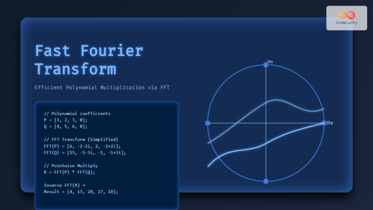
• P: [1, 2, 3, 0]
• Q: [4, 5, 6, 0]

2. Compute FFT of both padded polynomials

Calculate DFTs of arrays P and Q using FFT.

3. Pointwise Multiplication

Multiply the transformed values element-wise.

4. Compute Inverse FFT

Apply inverse FFT to get the resulting polynomial coefficients.

5. Result

The resulting coefficients correspond to the product polynomial R(x) = 4 + 13x + 28x^2 + 27x^3 + 18x^4.

Code Sample: Python Implementation of FFT Polynomial Multiplication

import cmath

def fft(a):
    n = len(a)
    if n == 1:
        return a
    even = fft(a[0::2])
    odd = fft(a[1::2])
    t = [cmath.exp(-2j * cmath.pi * k / n) * odd[k] for k in range(n // 2)]
    return [even[k] + t[k] for k in range(n // 2)] + \
           [even[k] - t[k] for k in range(n // 2)]

def ifft(a):
    n = len(a)
    a_conj = [x.conjugate() for x in a]
    y = fft(a_conj)
    return [x.conjugate() / n for x in y]

def poly_multiply(p, q):
    n = 1
    while n < len(p) + len(q) - 1:
        n <<= 1
    p += [0] * (n - len(p))
    q += [0] * (n - len(q))
    P = fft(p)
    Q = fft(q)
    R = [P[i] * Q[i] for i in range(n)]
    result = ifft(R)
    return [round(x.real) for x in result]

# Example:
p = [1, 2, 3]
q = [4, 5, 6]
print(poly_multiply(p, q))

This will output:

[4, 13, 28, 27, 18]

Why FFT Is Essential in Modern Computing

FFT-based multiplication is critical in many fields where fast polynomial or large integer multiplication matters, such as:

• Signal processing and audio/image compression
• Cryptography and coding theory
• Computational number theory and large integer arithmetic

Its logarithmic efficiency compared to naive approaches enables problems previously considered infeasible to be solved in real time.

Summary

The Fast Fourier Transform algorithm elegantly transforms the polynomial multiplication problem into pointwise multiplication via fast evaluation and interpolation using roots of unity. By combining divide-and-conquer recursion with complex number transformations, it drastically reduces computational complexity from quadratic to near-linear time.

This article has explained the theory behind FFT, shown a step-by-step example, included visual mermaid diagrams to clarify the workflow, and provided a Python implementation to solidify understanding.

Mastering FFT polynomial multiplication opens doors to efficient algorithms in many technical domains and is a fundamental tool in the computer scientist’s toolkit.