The Excel TRUNC function is a powerful mathematical tool that allows you to truncate decimal numbers by removing digits after a specified decimal place without rounding. Unlike the ROUND function, TRUNC simply cuts off digits, making it essential for precise financial calculations, data cleaning, and number formatting tasks.
What is the Excel TRUNC Function?
TRUNC stands for “truncate” and performs exactly what its name suggests – it truncates numbers by removing decimal places. This function is particularly valuable when you need to eliminate fractional parts of numbers without any rounding behavior that might alter your data’s accuracy.
The key difference between TRUNC and similar functions like ROUND or INT is that TRUNC never rounds up or down – it simply removes the specified decimal places, always moving the result closer to zero.
TRUNC Function Syntax and Parameters
The TRUNC function follows this straightforward syntax:
=TRUNC(number, [num_digits])
Parameters Explained:
- number (required): The numeric value you want to truncate
- num_digits (optional): Specifies how many digits to retain after the decimal point. Default is 0 if omitted
Parameter Behavior:
- When num_digits = 0: Truncates to a whole number
- When num_digits > 0: Retains the specified number of decimal places
- When num_digits < 0: Truncates digits to the left of the decimal point
Basic TRUNC Function Examples
Example 1: Simple Decimal Truncation
| Formula | Result | Explanation |
|---|---|---|
| =TRUNC(3.14159) | 3 | Removes all decimal places (default behavior) |
| =TRUNC(3.14159, 2) | 3.14 | Keeps 2 decimal places |
| =TRUNC(3.14159, 4) | 3.1415 | Keeps 4 decimal places |
Example 2: Working with Negative Numbers
| Formula | Result | Explanation |
|---|---|---|
| =TRUNC(-7.85) | -7 | Truncates toward zero, not down |
| =TRUNC(-7.85, 1) | -7.8 | Keeps 1 decimal place |
Advanced TRUNC Techniques
Truncating to the Left of Decimal Point
Using negative values for num_digits allows you to truncate digits to the left of the decimal point, effectively rounding down to the nearest ten, hundred, thousand, etc.
| Formula | Original Number | Result | Effect |
|---|---|---|---|
| =TRUNC(1234.56, -1) | 1234.56 | 1230 | Truncates to nearest ten |
| =TRUNC(1234.56, -2) | 1234.56 | 1200 | Truncates to nearest hundred |
| =TRUNC(1234.56, -3) | 1234.56 | 1000 | Truncates to nearest thousand |
TRUNC vs Other Excel Functions
TRUNC vs ROUND
Understanding the difference between TRUNC and ROUND is crucial for accurate data processing:
| Number | =TRUNC(number, 1) | =ROUND(number, 1) | Difference |
|---|---|---|---|
| 3.18 | 3.1 | 3.2 | ROUND rounds up, TRUNC cuts off |
| 3.14 | 3.1 | 3.1 | Same result when no rounding needed |
| -2.67 | -2.6 | -2.7 | Both move toward zero differently |
TRUNC vs INT
The INT function also removes decimal places, but behaves differently with negative numbers:
| Number | =TRUNC(number) | =INT(number) | Key Difference |
|---|---|---|---|
| 5.8 | 5 | 5 | Same for positive numbers |
| -5.8 | -5 | -6 | TRUNC toward zero, INT rounds down |
Practical Applications and Use Cases
Financial Calculations
TRUNC is invaluable in financial modeling where precise decimal control is required:
- Currency Conversion:
=TRUNC(A1*1.25, 2)for converting prices with 2 decimal precision - Tax Calculations:
=TRUNC(B1*0.08, 2)for calculating sales tax amounts - Discount Pricing:
=TRUNC(C1*0.85, 2)for applying percentage discounts
Data Cleaning and Standardization
Use TRUNC to standardize numeric data formats across datasets:
- Measurement Standardization:
=TRUNC(weight_in_kg, 1)to standardize weight measurements - Survey Data Processing:
=TRUNC(rating_score, 0)to convert decimal ratings to whole numbers - Performance Metrics:
=TRUNC(completion_percentage, 2)for consistent percentage reporting
Time and Date Calculations
TRUNC can help with time-based calculations by removing fractional days or hours:
- Age Calculations:
=TRUNC((TODAY()-birthdate)/365.25, 0)for whole number ages - Project Duration:
=TRUNC(end_date-start_date, 0)for complete days only
Common TRUNC Function Errors and Solutions
Error #1: #VALUE! Error
Cause: Non-numeric values in the number parameter
Solution: Use ISNUMBER() to check data types or VALUE() to convert text numbers
=IF(ISNUMBER(A1), TRUNC(A1, 2), "Invalid Number")
Error #2: Unexpected Results with Large Numbers
Cause: Excel’s floating-point precision limitations
Solution: Be aware of precision limits for very large numbers (15 significant digits)
Error #3: Negative Number Confusion
Cause: Misunderstanding how TRUNC handles negative numbers
Solution: Remember TRUNC always moves toward zero, not toward negative infinity
Advanced TRUNC Formulas and Combinations
Combining TRUNC with Other Functions
Create powerful data processing formulas by combining TRUNC with other Excel functions:
1. TRUNC with IF for Conditional Truncation
=IF(A1>100, TRUNC(A1, 0), TRUNC(A1, 2))
Truncates to whole numbers for values over 100, keeps 2 decimals otherwise
2. TRUNC with SUM for Aggregate Calculations
=SUM(TRUNC(A1:A10, 2))
Sums a range after truncating each value to 2 decimal places
3. TRUNC with AVERAGE for Statistical Analysis
=TRUNC(AVERAGE(B1:B20), 3)
Calculates average and truncates result to 3 decimal places
Performance Considerations and Best Practices
Optimization Tips
- Array Formulas: Use TRUNC in array formulas for processing multiple values efficiently
- Helper Columns: Consider helper columns for complex TRUNC calculations rather than nested formulas
- Conditional Formatting: Combine TRUNC with conditional formatting for visual data validation
Best Practices
- Document Your Logic: Always comment why you’re using TRUNC instead of ROUND
- Validate Results: Double-check TRUNC results, especially with negative numbers
- Consider Context: Choose between TRUNC, ROUND, and INT based on your specific needs
- Test Edge Cases: Verify behavior with zero, negative numbers, and very large values
Real-World Example: Sales Commission Calculator
Here’s a practical example showing how TRUNC can be used in a sales commission calculator:
| Sales Amount | Commission Rate | Raw Commission | Truncated Commission | Formula |
|---|---|---|---|---|
| $15,750 | 8.5% | $1,338.75 | $1,338.00 | =TRUNC(A2*B2, 0) |
| $23,400 | 12.3% | $2,878.20 | $2,878.20 | =TRUNC(A3*B3, 2) |
Alternative Methods and Workarounds
Using INT Instead of TRUNC
For positive numbers only, INT can substitute TRUNC:
=INT(A1*100)/100 // Equivalent to TRUNC(A1, 2) for positive numbers
Manual Truncation with Mathematical Operations
Create custom truncation logic using basic math:
=SIGN(A1)*INT(ABS(A1)*100)/100 // Manual 2-decimal truncation
Troubleshooting TRUNC Function Issues
Common Problems and Solutions
- Inconsistent Results Across Versions: TRUNC behavior is consistent across Excel versions, but formatting might differ
- Unexpected Rounding: If you see rounding, check if you’re actually using ROUND instead of TRUNC
- Scientific Notation Issues: Very large numbers might display in scientific notation; adjust cell formatting
- Precision Problems: For financial calculations, consider using specialized accounting functions
Conclusion
The Excel TRUNC function is an essential tool for precise number manipulation, offering exact control over decimal truncation without unwanted rounding. By understanding its syntax, behavior with negative numbers, and practical applications, you can leverage TRUNC for accurate financial calculations, data standardization, and professional spreadsheet development.
Whether you’re processing sales data, cleaning imported datasets, or performing complex mathematical operations, TRUNC provides the precision and reliability needed for professional Excel work. Practice with the examples provided, and experiment with combining TRUNC with other Excel functions to create powerful data processing solutions.
Remember that choosing between TRUNC, ROUND, and INT depends on your specific requirements – use TRUNC when you need exact truncation without any rounding behavior, ensuring your data maintains its intended precision throughout your calculations.
Related Posts

Excel INT Function: Complete Guide to Integer Extraction and Rounding
The Excel INT function is a fundamental mathematical function that extracts the integer portion of a number by rounding it...

Excel ROUNDDOWN Function: Master Downward Rounding with Precision Control
The Excel ROUNDDOWN function is a powerful mathematical tool that rounds numbers down toward zero to a specified number of...

Excel FLOOR Function: Complete Guide to Floor Rounding with Syntax Examples
The Excel FLOOR function is a powerful mathematical tool that rounds numbers down to the nearest specified multiple. Unlike standard...

JavaScript Math.trunc() Method: Integer Part
JavaScript Math.trunc() Method: Getting the Integer Part of a Number The Math.trunc() method in JavaScript is a built-in function that...

Excel ROUND Function: Complete Guide to Number Rounding in Spreadsheets
The Excel ROUND function is one of the most essential tools for managing numerical precision in spreadsheets. Whether you're working...

Excel ROUNDUP Function: Complete Guide to Upward Rounding with Formula Examples
The Excel ROUNDUP function is an essential tool for anyone working with numerical data in spreadsheets. Unlike standard rounding that...

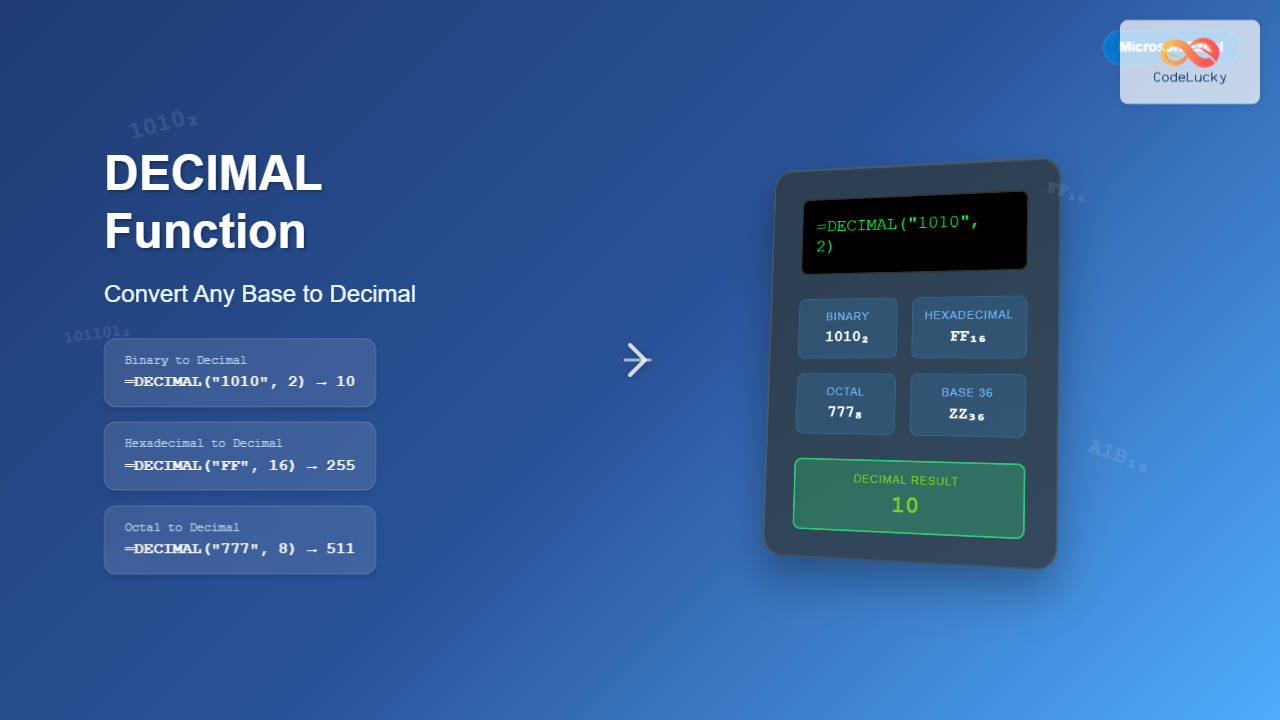
Excel DECIMAL Function: Convert Any Base Number to Decimal Instantly
The DECIMAL function in Excel is a powerful mathematical tool that converts numbers from any specified base to decimal (base...

Excel OCT2DEC Function: Complete Guide to Converting Octal Numbers to Decimal
What is the Excel OCT2DEC Function? The OCT2DEC function in Microsoft Excel is a powerful engineering function that converts octal...

Excel BASE Function: Complete Guide to Number Base Conversion
The BASE function in Excel is a powerful mathematical tool that converts decimal numbers into different number bases, making it...

Excel DEC2BIN Function: Complete Guide to Converting Decimal to Binary Numbers
What is the Excel DEC2BIN Function? The DEC2BIN function in Microsoft Excel is a powerful engineering function that converts decimal...

MySQL CEIL Function: Rounding Up Made Easy
The MySQL CEIL function, also known as CEILING, is a fundamental numeric function used to round a number up to...

Excel CEILING Function: Complete Guide to Rounding Up Numbers
The Excel CEILING function is a powerful mathematical tool that rounds numbers up to the nearest specified multiple. Whether you're...