What is the Excel IFNA Function?
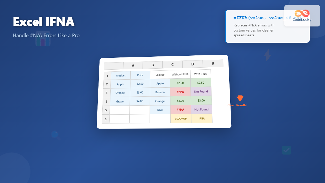
The IFNA function in Microsoft Excel is a powerful error-handling tool designed specifically to catch and manage #N/A (Not Available) errors in your spreadsheets. This function allows you to replace #N/A errors with custom values, making your data more presentable and your formulas more robust.
Unlike the generic IFERROR function, IFNA targets only #N/A errors, giving you precise control over how these specific errors are handled while allowing other error types to display normally.
IFNA Function Syntax and Parameters
The IFNA function follows a simple two-parameter syntax:
=IFNA(value, value_if_na)Parameters Breakdown:
- value (required): The expression or formula you want to test for #N/A errors
- value_if_na (required): The value to return if the first parameter results in #N/A error
The function evaluates the first parameter and returns its result if no #N/A error occurs. If an #N/A error is detected, it returns the second parameter instead.
When Does Excel Generate #N/A Errors?
Understanding when #N/A errors occur helps you identify where IFNA functions are most beneficial:
Common #N/A Error Scenarios:
- VLOOKUP failures: When lookup values aren’t found in the table
- HLOOKUP misses: Horizontal lookup functions unable to locate data
- INDEX/MATCH combinations: When MATCH function can’t find the lookup value
- XLOOKUP issues: Modern lookup function encountering missing data
- Array formula problems: When array operations can’t find corresponding values
- Manual NA() function calls: Intentionally inserted #N/A values
Basic IFNA Function Examples
Simple VLOOKUP Protection
Instead of displaying ugly #N/A errors when VLOOKUP fails:
=IFNA(VLOOKUP(A2,D:F,2,FALSE),"Not Found")This formula searches for the value in A2 within columns D through F, returning the second column’s value if found, or “Not Found” if the lookup fails.
INDEX/MATCH Error Handling
=IFNA(INDEX(B:B,MATCH(A2,C:C,0)),"No Match")This combination protects against #N/A errors when the MATCH function can’t locate the lookup value in column C.
Numerical Default Values
=IFNA(VLOOKUP(A2,data_table,3,0),0)Returns zero instead of #N/A when lookup operations fail, useful for mathematical calculations that need to continue despite missing data.
Advanced IFNA Applications
Nested IFNA Functions
You can nest multiple IFNA functions to create fallback lookup scenarios:
=IFNA(VLOOKUP(A2,table1,2,0),IFNA(VLOOKUP(A2,table2,2,0),"Not in either table"))This formula first searches table1, then table2 if the first lookup fails, finally displaying a message if neither lookup succeeds.
Combining IFNA with Other Functions
With CONCATENATE for Custom Messages:
=IFNA(VLOOKUP(A2,D:F,2,0),"Product " & A2 & " not found in database")With ISNUMBER for Validation:
=IF(ISNUMBER(A2),IFNA(VLOOKUP(A2,D:F,2,0),"ID not found"),"Invalid ID format")Dynamic Array Formulas with IFNA
In Excel 365 and Excel 2021, IFNA works seamlessly with dynamic arrays:
=IFNA(XLOOKUP(A2:A10,lookup_array,return_array),"Missing")This formula applies IFNA logic across an entire range, handling multiple lookups simultaneously.
IFNA vs IFERROR: Key Differences
While both functions handle errors, they serve different purposes:
| Aspect | IFNA | IFERROR |
|---|---|---|
| Error Types Handled | Only #N/A errors | All error types (#N/A, #VALUE!, #REF!, etc.) |
| Specificity | Highly specific | General purpose |
| Best Use Case | Lookup functions | General error prevention |
| Performance | Slightly faster for #N/A handling | More comprehensive but broader |
When to Choose IFNA:
- Working primarily with lookup functions
- Need to distinguish #N/A from other errors
- Want other error types to remain visible for debugging
- Building data validation scenarios
Real-World IFNA Use Cases
Sales Commission Calculator
=IFNA(VLOOKUP(B2,commission_table,2,0)*C2,"Base rate only")This formula calculates commissions based on a lookup table, applying a default message when specific commission rates aren’t found.
Inventory Management System
=IFNA(INDEX(stock_levels,MATCH(product_code,product_list,0)),"Out of Stock")Displays current stock levels or indicates when products aren’t in the inventory system.
Customer Data Enrichment
=IFNA(VLOOKUP(customer_id,customer_details,4,0),"New Customer")Enriches customer data by looking up additional information, marking unknown customers appropriately.
Performance Optimization Tips
Minimize Calculation Load
Place complex lookup formulas in helper columns rather than embedding them directly in IFNA functions:
Helper column: =VLOOKUP(A2,large_table,2,0)
Main formula: =IFNA(B2,"Not Found")
Use Exact Match When Possible
Always use FALSE or 0 for exact matches in lookup functions within IFNA to avoid unexpected results:
=IFNA(VLOOKUP(A2,D:F,2,FALSE),"No match")Consider Table References
Use structured table references for better performance and readability:
=IFNA(VLOOKUP([@Product],ProductTable[#All],2,0),"Product not listed")Common IFNA Mistakes and Solutions
Mistake 1: Using IFNA for All Errors
Wrong: Using IFNA when you need to catch division by zero errors
Right: Use IFERROR for comprehensive error handling, IFNA only for #N/A errors
Mistake 2: Ignoring Data Types
Wrong: =IFNA(VLOOKUP(A2,D:F,2,0),0) when column 2 contains text
Right: =IFNA(VLOOKUP(A2,D:F,2,0),"") for text columns
Mistake 3: Overcomplicating Nested Formulas
Wrong: Excessive nesting that’s hard to debug
Right: Break complex logic into separate helper columns
Testing and Debugging IFNA Formulas
Step-by-Step Approach:
- Test the base formula first: Ensure your lookup formula works correctly
- Verify data types: Check that lookup values and table data match types
- Check for hidden characters: Use TRIM and CLEAN functions if needed
- Test edge cases: Verify behavior with empty cells and unusual data
Debugging Techniques:
=IFNA(VLOOKUP(A2,D:F,2,0),"Debug: " & A2 & " not found")Include the lookup value in your error message to help identify problematic data.
Best Practices for IFNA Implementation
Consistency in Error Messages
Standardize your error messages across the spreadsheet:
- Use “Not Found” for missing lookup values
- Use “N/A” for intentionally blank results
- Use descriptive messages for business-specific scenarios
Documentation and Comments
Add comments to complex IFNA formulas explaining the business logic:
=IFNA(VLOOKUP(A2,Products,2,0),"Discontinued")
// Returns product name or marks as discontinued
Regular Formula Auditing
Periodically review your IFNA formulas to ensure they still serve their intended purpose as your data structure evolves.
Excel Version Compatibility
The IFNA function is available in:
- Excel 2013 and later versions
- Excel for Microsoft 365
- Excel Online
- Excel for Mac 2016 and later
For earlier Excel versions, you can achieve similar functionality using:
=IF(ISNA(VLOOKUP(A2,D:F,2,0)),"Not Found",VLOOKUP(A2,D:F,2,0))Conclusion
The IFNA function is an essential tool for creating professional, user-friendly spreadsheets. By specifically targeting #N/A errors, it provides precise control over error handling in lookup operations while maintaining the visibility of other error types for debugging purposes.
Master the IFNA function to transform error-prone spreadsheets into polished, professional documents that handle missing data gracefully and provide meaningful feedback to users. Whether you’re building simple lookup tables or complex data analysis systems, IFNA ensures your formulas remain robust and your results stay clean.
Remember to combine IFNA with proper data validation, consistent error messaging, and thorough testing to create spreadsheets that not only work correctly but also provide an excellent user experience.

