Divide and Conquer Algorithms: Break Problems into Subproblems

Divide and Conquer is one of the most important algorithm design paradigms in computer science. It provides a powerful way to solve complex problems by breaking them into smaller, more manageable subproblems, solving them independently, and then combining the results. Many foundational algorithms, including Merge Sort, Quick Sort, and even Fast Fourier Transform (FFT), are built on this strategy.

Table of Contents

What is Divide and Conquer?

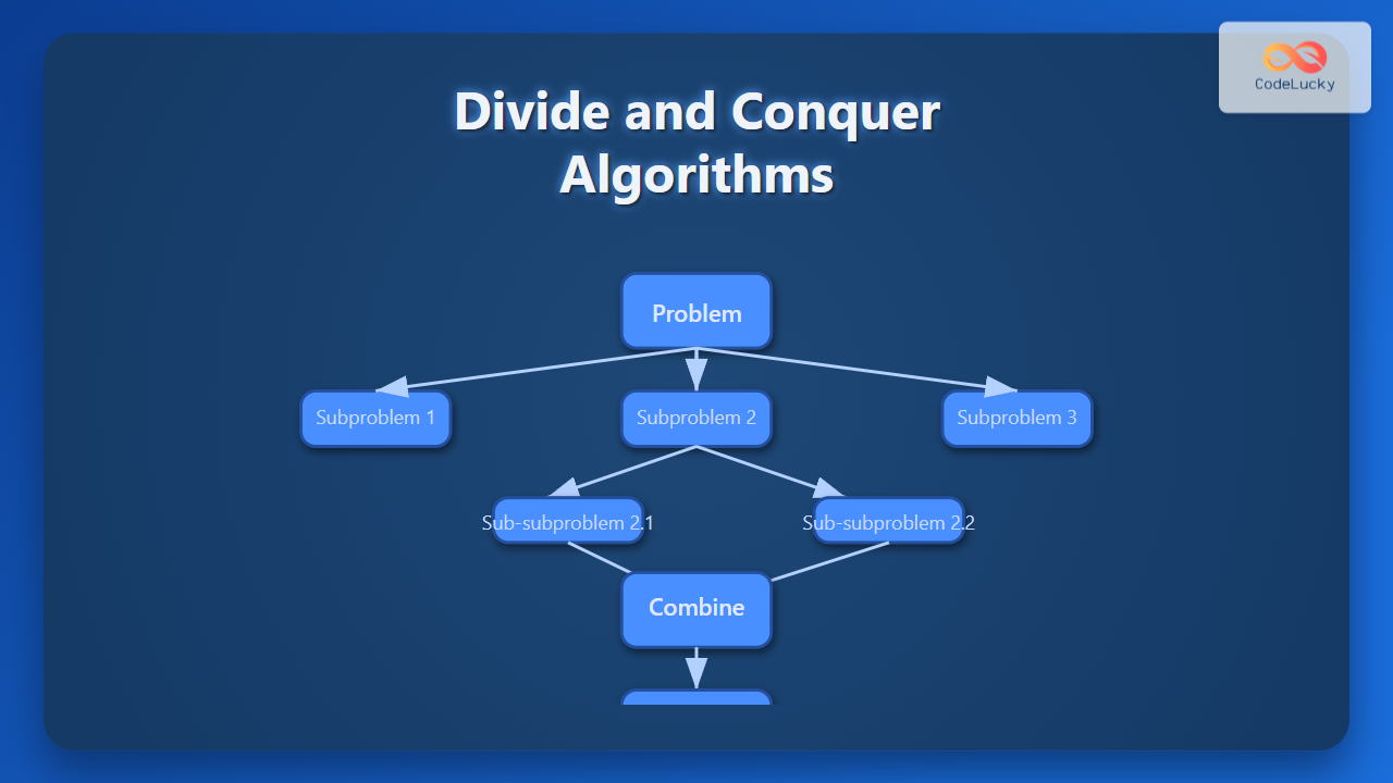
The core idea behind Divide and Conquer is simple yet effective. When faced with a large problem:

Divide: Break the problem into smaller subproblems.
Conquer: Solve the subproblems recursively (if they are still large, further divide them).
Combine: Merge the solutions of the subproblems to get the final answer.

Why Use Divide and Conquer?

Divide and Conquer algorithms provide several advantages:

Efficiency: They often reduce time complexity compared to naive approaches.
Scalability: Subproblems can be solved in parallel, making them suitable for parallel computing.
Simplification: Breaking problems down makes implementation and reasoning easier.

Examples of Divide and Conquer Algorithms

1. Merge Sort

Merge Sort is one of the classic algorithms that demonstrates Divide and Conquer in action:

Divide: Split the array into two halves.
Conquer: Recursively sort the two halves.
Combine: Merge the two sorted halves into one sorted array.

def merge_sort(arr):
    if len(arr) <= 1:
        return arr
    
    mid = len(arr) // 2
    left = merge_sort(arr[:mid])
    right = merge_sort(arr[mid:])
    
    return merge(left, right)

def merge(left, right):
    result = []
    i = j = 0
    while i < len(left) and j < len(right):
        if left[i] <= right[j]:
            result.append(left[i])
            i += 1
        else:
            result.append(right[j])
            j += 1
    result.extend(left[i:])
    result.extend(right[j:])
    return result

print(merge_sort([38, 27, 43, 3, 9, 82, 10]))

Output:

[3, 9, 10, 27, 38, 43, 82]

2. Quick Sort

Quick Sort improves sorting by using a pivot element:

Divide: Choose a pivot and partition the array into two subsets (less than pivot, greater than pivot).
Conquer: Recursively sort the two subsets.
Combine: Concatenate results.

def quick_sort(arr):
    if len(arr) <= 1:
        return arr
    
    pivot = arr[len(arr) // 2]
    left = [x for x in arr if x < pivot]
    middle = [x for x in arr if x == pivot]
    right = [x for x in arr if x > pivot]
    
    return quick_sort(left) + middle + quick_sort(right)

print(quick_sort([38, 27, 43, 3, 9, 82, 10]))

Output:

[3, 9, 10, 27, 38, 43, 82]

3. Binary Search

Binary Search is another Divide and Conquer algorithm used for searching in a sorted array:

Divide: Look at the middle element.
Conquer: If target is smaller, recurse into left half; if larger, recurse into right half.
Combine: Once the element is found, return its index.

def binary_search(arr, target):
    low, high = 0, len(arr) - 1
    
    while low <= high:
        mid = (low + high) // 2
        if arr[mid] == target:
            return mid
        elif arr[mid] < target:
            low = mid + 1
        else:
            high = mid - 1
    return -1

arr = [3, 9, 10, 27, 38, 43, 82]
print(binary_search(arr, 27))

Output:

Complexity of Divide and Conquer Algorithms

A general recurrence relation represents the time complexity of divide and conquer algorithms:

T(n) = aT(n/b) + f(n)

Where:

a: Number of subproblems
b: Size of subproblems (fraction of n)
f(n): Cost of dividing and combining

Using the Master Theorem, we can solve such recurrence relations efficiently. For example:

Merge Sort: T(n) = 2T(n/2) + O(n) = O(n log n)
Quick Sort (Average Case): T(n) = 2T(n/2) + O(n) = O(n log n)
Binary Search: T(n) = T(n/2) + O(1) = O(log n)

Real-World Applications

Data Compression: JPEG uses Divide and Conquer-based Discrete Cosine Transform.
Signal Processing: FFT for signal analysis.
Computational Geometry: Closest Pair of Points problem.
Scientific Computing: Matrix multiplication using Strassen’s Algorithm.

Conclusion

Divide and Conquer algorithms are more than just a programming concept—they form the backbone of optimization in computer science. By breaking problems into smaller parts, we not only improve efficiency but also gain clarity in problem-solving. Whether in sorting, searching, or scientific computations, this strategy continues to be an indispensable tool for programmers and researchers alike.