Dijkstra’s Algorithm is a fundamental algorithm in computer science used to find the shortest path between nodes in a weighted graph. This algorithm efficiently calculates the minimum distance from a starting node to every other node in the graph, making it invaluable in networking, mapping, and many real-world routing problems.
Understanding Dijkstra’s Algorithm
The core idea behind Dijkstra’s algorithm is to systematically explore nodes starting from a source, updating the shortest discovered distance to each node until the shortest paths to all nodes have been found.
The algorithm works only with non-negative weights on edges because it assumes once a shortest distance to a node is found, it cannot be improved further.
Algorithm Steps
- Initialize distances from the source to all nodes as
infinityexcept the source itself, which is zero. - Set of nodes whose shortest distance is finalized starts empty.
- Repeat until all nodes have been processed:
- Pick the unvisited node with the smallest tentative distance.
- For each neighbor of this node, calculate the distance from the source through the current node.
- If this distance is less than the current known distance, update it.
- Mark the current node as visited (finalized).
Example: Find Shortest Paths Using Dijkstra’s
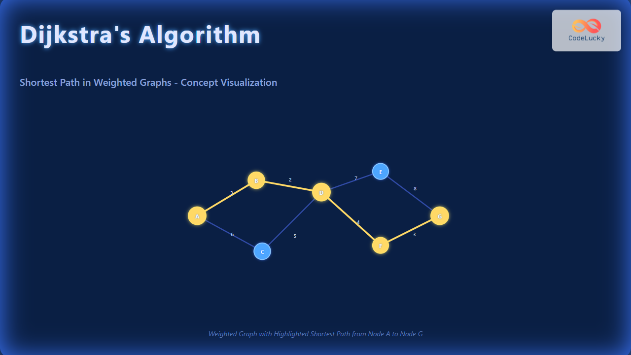
Consider the following weighted graph where numbers on edges represent distances:
We want the shortest path from node A to all others.
Step-by-Step Execution
| Node | Distance from A | Predecessor | Status |
|---|---|---|---|
| A | 0 | – | Visited |
| B | 3 | A | Unvisited |
| C | 1 | A | Unvisited |
| D | ∞ | – | Unvisited |
| E | ∞ | – | Unvisited |
1. Start with A. Distances to neighbors updated. Mark A visited.
2. Pick unvisited node with smallest distance: C (1). Update neighbors:
- D: min(∞, 1 + 2) = 3, predecessor = C
- E: min(∞, 1 + 4) = 5, predecessor = C
3. Next pick D (3). Update neighbors:
- E: min(5, 3 + 7) = 5 (unchanged)
4. Next pick B (3). Update neighbors:
- D: min(3, 3 + 7) = 3 (unchanged)
- C: min(1, 3 + 5) = 1 (unchanged)
5. Finally pick E (5). All nodes visited.
Final Table
| Node | Final Distance from A | Path |
|---|---|---|
| A | 0 | A |
| B | 3 | A → B |
| C | 1 | A → C |
| D | 3 | A → C → D |
| E | 5 | A → C → E |
Interactive Python Example
Below is a Python code snippet implementing Dijkstra’s Algorithm. This can be run locally or in any Python environment to observe the shortest path outputs.
import heapq

def dijkstra(graph, start):
    pq = [(0, start)]
    distances = {node: float('inf') for node in graph}
    distances[start] = 0
    predecessors = {node: None for node in graph}

    while pq:
        current_distance, current_node = heapq.heappop(pq)

        if current_distance > distances[current_node]:
            continue

        for neighbor, weight in graph[current_node].items():
            distance = current_distance + weight
            if distance < distances[neighbor]:
                distances[neighbor] = distance
                predecessors[neighbor] = current_node
                heapq.heappush(pq, (distance, neighbor))

    return distances, predecessors

# Example graph as adjacency list with weights
graph = {
    'A': {'B': 3, 'C': 1},
    'B': {'D': 7, 'C': 5},
    'C': {'D': 2, 'E': 4},
    'D': {'E': 7},
    'E': {}
}

distances, predecessors = dijkstra(graph, 'A')
print("Shortest distances:", distances)
print("Predecessors:", predecessors)
Time Complexity and Use Cases
Dijkstra’s algorithm time complexity depends on the data structures used. Using a min-priority queue (typically a binary heap), complexity is O((V + E) log V), where V is nodes count and E is edges count. It is efficient for sparse to moderately dense graphs.
Common use cases include GPS systems, network routing protocols, and various scheduling and optimization problems involving weighted paths.
Limitations and Alternatives
This algorithm does not work correctly if the graph contains negative weight edges. For such cases, the Bellman-Ford algorithm is preferred. For graphs where all edge weights are equal, a simple Breadth-First Search (BFS) can find shortest paths.
Summary
Dijkstra’s algorithm is a core graph algorithm for finding shortest paths in weighted graphs without negative edges. With clear steps, good performance, and wide use cases, it is essential knowledge for programmers and computer scientists dealing with pathfinding problems.
Understanding its design, implementation, and limitations ensures effective application in practical scenarios like routing, network design, and optimization.


