Device scheduling is a critical component of operating system design that determines how I/O requests are ordered and executed to optimize system performance. As storage devices like hard disk drives (HDDs) involve mechanical components with significant seek times, efficient scheduling algorithms can dramatically improve throughput and reduce response times.
Understanding I/O Request Scheduling
I/O request scheduling involves managing the order in which read and write operations are performed on storage devices. The primary goal is to minimize the total seek time – the time required for the disk head to move between different tracks on the disk surface.
When multiple processes make I/O requests simultaneously, the operating system must decide which request to service first. Poor scheduling can lead to excessive head movement, reduced throughput, and increased latency.

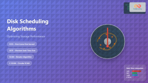
First-Come, First-Served (FCFS) Algorithm
The First-Come, First-Served (FCFS) algorithm is the simplest I/O scheduling method. Requests are processed in the exact order they arrive in the queue, without any optimization for seek time reduction.
FCFS Algorithm Implementation
The FCFS algorithm follows these steps:
- Accept incoming I/O requests in arrival order
- Place requests in a FIFO queue
- Process requests sequentially from the front of the queue
- Complete each request before moving to the next
FCFS Example
Consider a disk with 200 tracks (0-199) and the current head position at track 50. The request queue contains: [82, 170, 43, 140, 24, 16, 190].
FCFS Processing Order:
- Start: 50 → 82 (seek distance: 32)
- 82 → 170 (seek distance: 88)
- 170 → 43 (seek distance: 127)
- 43 → 140 (seek distance: 97)
- 140 → 24 (seek distance: 116)
- 24 → 16 (seek distance: 8)
- 16 → 190 (seek distance: 174)
Total seek distance: 32 + 88 + 127 + 97 + 116 + 8 + 174 = 642 tracks
FCFS Advantages and Disadvantages
Advantages:
- Simple implementation with minimal overhead
- Fair scheduling – no request starvation
- Predictable behavior
Disadvantages:
- Poor performance due to random seek patterns
- High average seek time
- No optimization for disk geometry
Shortest Seek Time First (SSTF) Algorithm
The Shortest Seek Time First (SSTF) algorithm improves upon FCFS by selecting the request that requires the minimum seek distance from the current head position.
SSTF Algorithm Implementation
The SSTF algorithm operates as follows:
- Calculate seek distance for all pending requests
- Select the request with minimum seek distance
- Service the selected request
- Update current head position
- Repeat until all requests are processed
SSTF Example
Using the same scenario: disk with 200 tracks, head at position 50, requests: [82, 170, 43, 140, 24, 16, 190].
SSTF Processing Order:
- Start: 50 → 43 (distance: 7, closest to 50)
- 43 → 24 (distance: 19, closest to 43)
- 24 → 16 (distance: 8, closest to 24)
- 16 → 82 (distance: 66, closest to 16)
- 82 → 140 (distance: 58, closest to 82)
- 140 → 170 (distance: 30, closest to 140)
- 170 → 190 (distance: 20, closest to 170)
Total seek distance: 7 + 19 + 8 + 66 + 58 + 30 + 20 = 208 tracks
SSTF reduces seek distance by 67% compared to FCFS!
SSTF Advantages and Disadvantages
Advantages:
- Significant reduction in average seek time
- Better throughput than FCFS
- Relatively simple implementation
Disadvantages:
- Can cause starvation of requests far from current position
- Not optimal for all scenarios
- May lead to unfair service distribution
SCAN (Elevator) Algorithm
The SCAN algorithm, also known as the elevator algorithm, moves the disk head in one direction, servicing all requests in that direction until reaching the disk boundary, then reverses direction.

SCAN Algorithm Implementation
The SCAN algorithm follows these steps:
- Determine initial direction of head movement
- Service all requests in the current direction
- Continue until reaching disk boundary
- Reverse direction and repeat
- Complete when all requests are serviced
SCAN Example
Same scenario: head at position 50, moving toward higher tracks, requests: [82, 170, 43, 140, 24, 16, 190].
SCAN Processing Order (moving up then down):
- Start: 50 → 82 (distance: 32)
- 82 → 140 (distance: 58)
- 140 → 170 (distance: 30)
- 170 → 190 (distance: 20)
- 190 → 199 (distance: 9, reach boundary)
- 199 → 43 (distance: 156, reverse direction)
- 43 → 24 (distance: 19)
- 24 → 16 (distance: 8)
Total seek distance: 32 + 58 + 30 + 20 + 9 + 156 + 19 + 8 = 332 tracks
SCAN Advantages and Disadvantages
Advantages:
- Prevents starvation of requests
- Predictable seek patterns
- Good performance for heavy I/O loads
- Fair distribution of service
Disadvantages:
- Unnecessary movement to disk boundaries
- Longer wait times for requests at opposite ends
- Not optimal for light I/O loads
C-SCAN (Circular SCAN) Algorithm
The C-SCAN algorithm is a variation of SCAN that provides more uniform wait times. Instead of reversing direction, the head returns to the beginning of the disk and continues in the same direction.
C-SCAN Algorithm Implementation
C-SCAN operates with these principles:
- Move head in one direction only (typically increasing)
- Service all requests encountered in that direction
- Upon reaching the end, return to the beginning
- Continue servicing in the same direction
- Treat disk as circular
C-SCAN Example
Using our scenario: head at 50, moving toward higher tracks, requests: [82, 170, 43, 140, 24, 16, 190].
C-SCAN Processing Order:
- Start: 50 → 82 (distance: 32)
- 82 → 140 (distance: 58)
- 140 → 170 (distance: 30)
- 170 → 190 (distance: 20)
- 190 → 199 (distance: 9, reach end)
- 199 → 0 (distance: 199, return to start)
- 0 → 16 (distance: 16)
- 16 → 24 (distance: 8)
- 24 → 43 (distance: 19)
Total seek distance: 32 + 58 + 30 + 20 + 9 + 199 + 16 + 8 + 19 = 391 tracks
C-SCAN Advantages and Disadvantages
Advantages:
- More uniform wait times than SCAN
- Eliminates bias against requests at disk ends
- Predictable service patterns
- No starvation issues
Disadvantages:
- Higher seek distance due to return trips
- Wasted movement during repositioning
- Complex implementation
LOOK and C-LOOK Algorithms
The LOOK and C-LOOK algorithms are optimized versions of SCAN and C-SCAN respectively. Instead of moving to disk boundaries, they only move as far as the furthest request in each direction.

LOOK Algorithm Example
Same scenario with LOOK algorithm moving upward first:
LOOK Processing Order:
- Start: 50 → 82 (distance: 32)
- 82 → 140 (distance: 58)
- 140 → 170 (distance: 30)
- 170 → 190 (distance: 20, furthest request)
- 190 → 43 (distance: 147, reverse direction)
- 43 → 24 (distance: 19)
- 24 → 16 (distance: 8, furthest request down)
Total seek distance: 32 + 58 + 30 + 20 + 147 + 19 + 8 = 314 tracks
C-LOOK Algorithm Example
C-LOOK Processing Order:
- Start: 50 → 82 (distance: 32)
- 82 → 140 (distance: 58)
- 140 → 170 (distance: 30)
- 170 → 190 (distance: 20)
- 190 → 16 (distance: 174, jump to lowest)
- 16 → 24 (distance: 8)
- 24 → 43 (distance: 19)
Total seek distance: 32 + 58 + 30 + 20 + 174 + 8 + 19 = 341 tracks
Performance Comparison and Analysis
Let’s compare the performance of all algorithms using our example scenario:
| Algorithm | Total Seek Distance | Average Seek Distance | Performance Rank |
|---|---|---|---|
| FCFS | 642 tracks | 91.7 tracks | 6 (Worst) |
| SSTF | 208 tracks | 29.7 tracks | 1 (Best) |
| SCAN | 332 tracks | 47.4 tracks | 3 |
| C-SCAN | 391 tracks | 55.9 tracks | 5 |
| LOOK | 314 tracks | 44.9 tracks | 2 |
| C-LOOK | 341 tracks | 48.7 tracks | 4 |

Real-World Applications and Considerations
Modern Storage Systems
While these algorithms were designed for traditional HDDs, modern storage systems present new challenges:
- Solid State Drives (SSDs): No mechanical seek time, making position-based scheduling less relevant
- RAID Arrays: Multiple disks require coordinated scheduling
- Network Storage: Network latency becomes a significant factor
Operating System Implementation
Most modern operating systems implement hybrid approaches:
- Linux: Uses CFQ (Completely Fair Queuing) and deadline schedulers
- Windows: Employs elevator-based algorithms with fairness modifications
- macOS: Implements adaptive scheduling based on workload characteristics
Algorithm Selection Guidelines
Choose SSTF when:
- Maximum throughput is the primary concern
- Request patterns are relatively uniform
- Starvation is not a critical issue
Choose SCAN/LOOK when:
- Fairness and starvation prevention are important
- System has heavy, continuous I/O load
- Predictable response times are required
Choose C-SCAN/C-LOOK when:
- Uniform response times across all track positions
- High-priority applications require consistent performance
- System serves diverse workloads
Implementation Considerations
Queue Management
Effective I/O scheduling requires sophisticated queue management:
- Priority Queues: Separate queues for different request types
- Aging Mechanisms: Prevent starvation by gradually increasing request priority
- Deadline Scheduling: Ensure time-critical requests meet their deadlines
Performance Optimization
Several techniques can enhance scheduling performance:
- Request Merging: Combine adjacent requests to reduce overhead
- Read-ahead Caching: Anticipate future requests based on access patterns
- Write Coalescing: Batch multiple write operations
- Elevator Sorting: Maintain requests in sorted order for efficient processing
Future Trends and Developments
I/O scheduling continues to evolve with emerging technologies:
- NVMe and Storage Class Memory: Ultra-low latency devices requiring new scheduling paradigms
- AI-Driven Scheduling: Machine learning algorithms that adapt to workload patterns
- Distributed Storage: Scheduling across multiple nodes and data centers
- Quality of Service (QoS): Guaranteed performance levels for different application types
Understanding these I/O request scheduling algorithms is essential for system administrators, developers, and anyone working with storage systems. Each algorithm offers different trade-offs between performance, fairness, and complexity. The choice depends on specific system requirements, workload characteristics, and performance objectives. Modern systems often employ hybrid approaches that combine multiple algorithms to achieve optimal performance across diverse scenarios.
Related Posts
Disk Scheduling Algorithms: FCFS, SSTF, SCAN, C-SCAN – Complete Implementation Guide
Disk scheduling algorithms are fundamental components of operating systems that determine the order in which disk I/O requests are processed....
ionice Command Linux: Master IO Scheduling Priority for Optimal System Performance
The ionice command is a powerful Linux utility that allows system administrators and developers to control the Input/Output (IO) scheduling...

Process Scheduling in Operating System: Algorithms, Types & Implementation Guide
Process scheduling is one of the most critical components of an operating system that determines how the CPU time is...

Spooling in OS: Complete Guide to Simultaneous Peripheral Operations Online
What is Spooling in Operating System? Spooling (Simultaneous Peripheral Operations Online) is a fundamental technique in operating systems that enables...

Log-structured File System: Sequential Write Optimization for High-Performance Storage
Log-structured File Systems (LFS) represent a revolutionary approach to data storage that fundamentally changes how operating systems handle file operations....

Multilevel Queue Scheduling: Multiple Priority Levels in Operating Systems
Introduction to Multilevel Queue Scheduling Multilevel queue scheduling is a sophisticated CPU scheduling algorithm used in operating systems to manage...
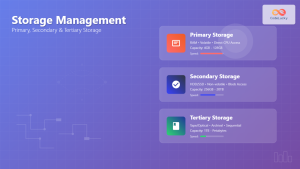
Storage Management: Complete Guide to Primary, Secondary and Tertiary Storage Systems
Storage management is one of the most critical components of an operating system, responsible for efficiently organizing, accessing, and maintaining...

CPU Scheduling Algorithms: FCFS, SJF, Round Robin Complete Guide
CPU scheduling is a fundamental concept in operating systems that determines how processes are allocated processor time. The CPU scheduler...

Virtual CPU Scheduling: Complete Guide to Time-sharing Physical Processors
Virtual CPU scheduling is the cornerstone of modern operating systems, enabling multiple processes to share limited physical processors efficiently. This...

Buffering in Operating System: Complete Guide to Single, Double and Circular Buffer Implementation
What is Buffering in Operating System? Buffering in operating systems is a fundamental technique used to temporarily store data in...

Priority Scheduling Algorithm: Complete Implementation Guide with Examples
What is Priority Scheduling Algorithm? Priority scheduling is a CPU scheduling algorithm where each process is assigned a priority value,...

Round Robin Scheduling: Time Quantum and Performance Analysis in Operating Systems
What is Round Robin Scheduling? Round Robin (RR) scheduling is a preemptive CPU scheduling algorithm that assigns equal time slices,...