Decision Tree Algorithm: Interpretable Classification Method Explained with Examples

The Decision Tree Algorithm is one of the most popular and interpretable machine learning algorithms used for classification and regression problems. Unlike black-box models such as neural networks, decision trees provide clear visibility into how predictions are made. In this article, we will explore the decision tree algorithm in depth, discuss how it works, review core concepts like entropy and information gain, and provide examples with intuitive visualizations.

What is a Decision Tree Algorithm?

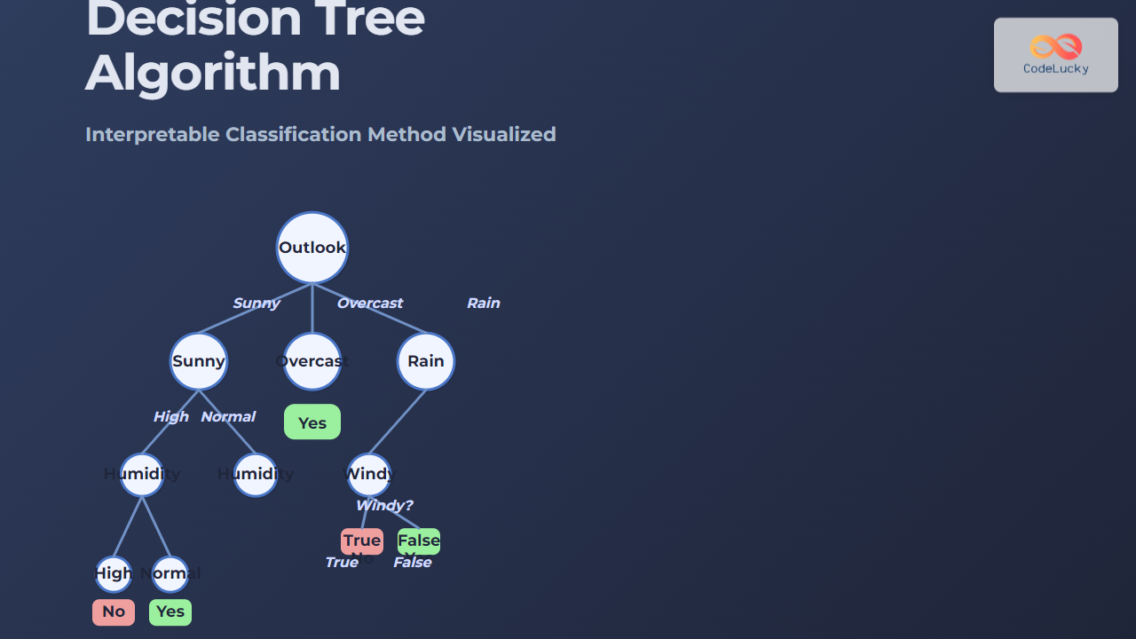
A decision tree is a flowchart-like tree structure in which each internal node represents a test on a feature, each branch represents the outcome of the test, and each leaf node represents a class label or prediction. This makes it easy to interpret, since the decision path for a sample can be traced from the root to the leaf.

Key Concepts in Decision Trees

• Root Node: The top-most node representing the entire dataset split on the best attribute.
• Splitting: The process of dividing data records into subsets based on a feature value.
• Leaf Node: Terminal nodes that represent class labels or predictions.
• Entropy: A measure of impurity in the dataset.
• Information Gain: The reduction in entropy achieved by partitioning the dataset on a given attribute.
• Gini Index: An alternative to entropy used to measure impurity.

Mathematical Foundation

The efficiency of a decision tree largely depends on how we measure purity of a split. The most common criteria are:

1. Entropy

Entropy quantifies the uncertainty in data:

Entropy(S) = - Σ p_i * log₂(p_i)

where p_i is the probability of class i in dataset S.

2. Information Gain

Information Gain is the reduction in entropy after splitting the dataset on an attribute:

Information Gain(S, A) = Entropy(S) - Σ (|S_v|/|S|) * Entropy(S_v)

3. Gini Index

An alternative criterion used in CART (Classification and Regression Trees):

Gini(S) = 1 - Σ p_i²

Example: Weather-Based Classification

Consider a simple classification problem: predicting whether a person will play tennis based on weather conditions.

Outlook	Temperature	Humidity	Windy	Play Tennis
Sunny	Hot	High	False	No
Overcast	Hot	High	False	Yes
Rain	Mild	High	False	Yes
Sunny	Mild	High	True	No

When building a decision tree, the algorithm evaluates which feature (Outlook, Temperature, Humidity, Windy) provides the highest information gain. In this example, Outlook is likely the best root feature.

Advantages of Decision Trees

• Highly interpretable and explainable.
• Does not require feature scaling or normalization.
• Can handle both numerical and categorical data.
• Performs automatic feature selection based on information gain or Gini index.

Limitations of Decision Trees

• Prone to overfitting if not pruned properly.
• Small variations in data may lead to significant structural changes in the tree.
• Not suitable for datasets with too many features without feature importance analysis.

Practical Implementation Using Python

Here’s a quick example using scikit-learn:

from sklearn import datasets
from sklearn.tree import DecisionTreeClassifier, plot_tree
import matplotlib.pyplot as plt

# Load dataset
iris = datasets.load_iris()
X, y = iris.data, iris.target

# Train Decision Tree
clf = DecisionTreeClassifier(criterion="entropy", max_depth=3)
clf.fit(X, y)

# Visualize
plt.figure(figsize=(12, 8))
plot_tree(clf, feature_names=iris.feature_names, class_names=iris.target_names, filled=True)
plt.show()

This produces a clear visualization of splits based on petal length, petal width, and other features of the famous Iris dataset.

Interactive Conceptual Visualization

Imagine you are deciding whether to buy a laptop. You might ask:

1. Is the price within budget?
2. If yes: Is the brand trusted?
3. If yes: You buy it. Else: You skip it.

Optimizing Decision Trees

Overfitting is a common concern in decision trees. Techniques to optimize include:

• Pruning: Reduces overfitting by removing unnecessary branches.
• Setting Max Depth: Restricts the maximum levels of the tree.
• Minimum Samples per Leaf: Stops splitting when nodes have too few samples.
• Ensemble Methods: Combine multiple trees for better accuracy (e.g., Random Forests, Gradient Boosted Trees).

Real-World Applications

• Healthcare: Diagnosing diseases based on patient symptoms.
• Finance: Credit risk assessment and loan approval automation.
• Marketing: Customer segmentation and predictive lead scoring.
• Manufacturing: Quality inspection and defect detection.

Conclusion

The Decision Tree Algorithm stands out as a highly interpretable classification method that balances simplicity with strong predictive power. While it may struggle with overfitting, when optimized or combined with ensemble methods, it becomes a versatile tool widely adopted in various real-world domains. For data scientists and engineers seeking interpretable machine learning models, decision trees remain a top choice.