The Bellman-Ford algorithm is a fundamental graph algorithm used to find the shortest path from a single source vertex to all other vertices in a weighted graph. Unlike Dijkstra’s algorithm, Bellman-Ford can handle graphs with negative weight edges, making it a versatile and widely used algorithm in computer science and programming. This article delves deeply into the theory, working, and applications of the Bellman-Ford algorithm, accompanied by clear examples, visual explanations, and interactive code snippets to clarify each step of the process.
Understanding Bellman-Ford Algorithm
The Bellman-Ford algorithm operates by iteratively relaxing edges, thereby progressively shortening the estimated distance from the source to each vertex. It is capable of detecting negative weight cycles—cycles where the total weight is negative—highlighting if shortest paths do not exist because the cost can continually decrease. This makes Bellman-Ford invaluable in scenarios where negative weights are present, such as currency exchange arbitrage or routing protocols.
Key Properties
- Works with both positive and negative edge weights.
- Time complexity: O(V × E), where V is vertices count and E is edges count.
- Detects negative weight cycles reachable from the source.
Step-by-Step Working of Bellman-Ford
Given a graph G = (V, E) and a source vertex s, the algorithm proceeds as follows:
- Initialize: Set distance to source vertex as 0 and all others as infinity.
- Relax edges: Repeat for (V-1) times: For each edge (u, v) with weight w, update the distance to v as min(distance[v], distance[u] + w).
- Negative cycle check: Check all edges once again; if any distance can still be updated, report a negative weight cycle.
Example: Illustrative Graph
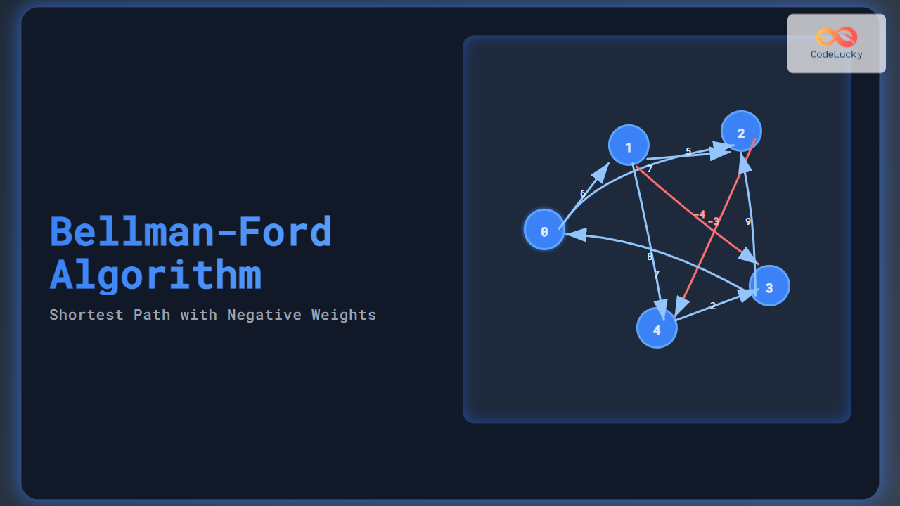
Consider this graph with 5 vertices (0 to 4) and weighted edges, some of which have negative weights:
Source vertex is 0. The goal is to find shortest paths from vertex 0 to all others.
Initialization:
- dist[0] = 0
- dist[1], dist[2], dist[3], dist[4] = ∞ (infinity)
Relax edges in iterations:
| Iteration | Distance Array (dist[]) | Explanation |
|---|---|---|
| 0 (initial) | [0, ∞, ∞, ∞, ∞] | Set source distance zero; others infinite. |
| 1 | [0, 6, 7, 2, 4] | Relax edges: from 0 to 1 (6), 0 to 2 (7), edge 1 to 3 with weight -4 etc. |
| 2 | [0, 6, 7, 2, 4] | No further changes, distances stabilize. |
The shortest paths from vertex 0 to others are finalized after V-1 iterations.
Code Example in Python
def bellman_ford(graph, V, src):
    dist = [float('inf')] * V
    dist[src] = 0

    for _ in range(V - 1):
        for u, v, w in graph:
            if dist[u] != float('inf') and dist[u] + w < dist[v]:
                dist[v] = dist[u] + w

    # Check for negative weight cycles
    for u, v, w in graph:
        if dist[u] != float('inf') and dist[u] + w < dist[v]:
            return "Graph contains negative weight cycle"

    return dist

# Graph edges: (u, v, w)
graph = [
    (0, 1, 6), (0, 2, 7), (1, 2, 5),
    (1, 3, -4), (1, 4, 8), (2, 4, -3),
    (3, 2, 9), (3, 0, 7), (4, 3, 2)
]

V = 5
src = 0

print(bellman_ford(graph, V, src))
This implementation clearly demonstrates how edges are relaxed and how the algorithm detects negative cycles.
Why Use Bellman-Ford Over Dijkstra?
- Negative edge weights: Dijkstra’s algorithm cannot handle negative weights reliably, whereas Bellman-Ford can.
- Cycle detection: Bellman-Ford detects negative weight cycles unreachable by Dijkstra’s approach.
Interactive Visualization Suggestion
For deeper learning, an interactive step-by-step relaxation visualization can be built using JavaScript or Python visualization libraries. Students can modify edge weights and see relaxation iterations in real time. This hands-on approach solidifies intuitive understanding.
Time and Space Complexity
- Time Complexity: O(V × E), due to the (V-1) iterations over E edges.
- Space Complexity: O(V) for storing distance array.
Additional Bellman-Ford Applications
- Routing algorithms in computer networks like RIP (Routing Information Protocol).
- Currency conversion and arbitrage detection in financial systems.
- Detecting feasible paths in road networks with tolls or penalties.
Summary
The Bellman-Ford algorithm is a crucial algorithm for shortest paths in graphs that may contain negative weight edges. Its ability to detect negative cycles and work with such edges makes it indispensable in certain real-world applications. Understanding its iterative edge relaxation gives deep insight into shortest path computations.
The combination of theoretical understanding, code examples, and visual diagrams makes mastering Bellman-Ford easier for programmers and algorithm learners alike.

