The Banker’s Algorithm is a fundamental deadlock avoidance algorithm in operating systems, designed to ensure that resource allocation maintains the system in a safe state. Named after the banking principle of maintaining sufficient reserves, this algorithm prevents deadlocks by carefully analyzing resource requests before granting them.
Understanding the Banker’s Algorithm
Developed by Edsger Dijkstra, the Banker’s Algorithm simulates the allocation of predetermined maximum resources to processes and determines whether the system can remain in a safe state after each allocation. The algorithm maintains several data structures to track current allocations, maximum needs, and available resources.

Key Data Structures
The Banker’s Algorithm relies on three primary matrices and one vector:
Available Vector (Available[m])
Represents the number of available instances of each resource type. If Available[j] = k, then k instances of resource type Rj are available.
Max Matrix (Max[n][m])
Defines the maximum demand of each process for each resource type. If Max[i][j] = k, then process Pi may request at most k instances of resource type Rj.
Allocation Matrix (Allocation[n][m])
Shows the number of resources of each type currently allocated to each process. If Allocation[i][j] = k, then process Pi is currently allocated k instances of resource type Rj.
Need Matrix (Need[n][m])
Represents the remaining resource need of each process. Calculated as: Need[i][j] = Max[i][j] - Allocation[i][j]
Safe State Concept
A system state is considered safe if there exists a sequence of processes (called a safe sequence) such that:
- For each process Pi in the sequence, the resources that Pi can still request can be satisfied by currently available resources plus resources held by all processes Pj where j < i
- If Pi‘s resource needs cannot be immediately satisfied, it can wait until all processes Pj (where j < i) have completed and released their resources

Algorithm Implementation
Safety Algorithm
The safety algorithm determines if the current system state is safe:
1. Initialize Work = Available and Finish[i] = false for all i
2. Find an index i such that:
   - Finish[i] == false
   - Need[i] <= Work
3. If no such i exists, go to step 5
4. Set Work = Work + Allocation[i] and Finish[i] = true
5. If Finish[i] == true for all i, the system is in a safe state
Resource-Request Algorithm
When process Pi requests resources represented by Requesti:
1. If Request[i] <= Need[i], go to step 2; otherwise, raise error
2. If Request[i] <= Available, go to step 3; otherwise, P[i] must wait
3. Pretend to allocate requested resources:
   Available = Available - Request[i]
   Allocation[i] = Allocation[i] + Request[i]
   Need[i] = Need[i] - Request[i]
4. If the resulting state is safe, complete the allocation
5. If unsafe, restore the original state and make P[i] wait
Detailed Example
Consider a system with 5 processes (P0-P4) and 3 resource types (A, B, C):
Initial System State
| Process | Allocation (A,B,C) | Max (A,B,C) | Need (A,B,C) |
|---|---|---|---|
| P0 | (0,1,0) | (7,5,3) | (7,4,3) |
| P1 | (2,0,0) | (3,2,2) | (1,2,2) |
| P2 | (3,0,2) | (9,0,2) | (6,0,0) |
| P3 | (2,1,1) | (2,2,2) | (0,1,1) |
| P4 | (0,0,2) | (4,3,3) | (4,3,1) |
Available Resources: (3,3,2)
Safety Check Process

Step-by-Step Safety Verification
Step 1: Work = (3,3,2), all Finish[i] = false
Step 2: Find process where Need ≤ Work
- P1: Need(1,2,2) ≤ Work(3,3,2) ✓
- Work = (3,3,2) + (2,0,0) = (5,3,2), Finish[1] = true
Step 3: Continue with updated Work
- P3: Need(0,1,1) ≤ Work(5,3,2) ✓
- Work = (5,3,2) + (2,1,1) = (7,4,3), Finish[3] = true
Step 4: Continue the process
- P4: Need(4,3,1) ≤ Work(7,4,3) ✓
- Work = (7,4,3) + (0,0,2) = (7,4,5), Finish[4] = true
Step 5: Continue
- P2: Need(6,0,0) ≤ Work(7,4,5) ✓
- Work = (7,4,5) + (3,0,2) = (10,4,7), Finish[2] = true
Step 6: Final check
- P0: Need(7,4,3) ≤ Work(10,4,7) ✓
- Work = (10,4,7) + (0,1,0) = (10,5,7), Finish[0] = true
Safe Sequence: <P1, P3, P4, P2, P0>
Resource Request Example
Suppose process P1 requests (1,0,2). Let’s check if this request can be granted:
Request Validation
Request[1] = (1,0,2)
Need[1] = (1,2,2)

Check: Request[1] <= Need[1]
(1,0,2) <= (1,2,2) ✓

Check: Request[1] <= Available
(1,0,2) <= (3,3,2) ✓
Temporary Allocation
| Matrix | Before | After |
|---|---|---|
| Available | (3,3,2) | (2,3,0) |
| Allocation[1] | (2,0,0) | (3,0,2) |
| Need[1] | (1,2,2) | (0,2,0) |

Safety Check After Request
With the new state, we verify safety:
- Available: (2,3,0)
- Find P3: Need(0,1,1) > Available(2,3,0) at resource C ✗
- Find P1: Need(0,2,0) ≤ Available(2,3,0) ✓
After P1 completes: Available = (2,3,0) + (3,0,2) = (5,3,2)
Continue with P3, P4, P2, P0… The system remains safe, so the request is granted.
Implementation in Pseudocode
function isSafe(available, max, allocation, processes, resources):
    need = calculateNeed(max, allocation)
    work = available.copy()
    finish = [false] * processes
    safeSequence = []

    count = 0
    while count < processes:
        found = false
        for i in range(processes):
            if not finish[i] and need[i] <= work:
                work += allocation[i]
                finish[i] = true
                safeSequence.append(i)
                found = true
                count += 1
                break

        if not found:
            return false, []

    return true, safeSequence

function requestResources(processId, request, available, max, allocation):
    need = calculateNeed(max, allocation)

    if request > need[processId]:
        return "Error: Request exceeds maximum claim"

    if request > available:
        return "Process must wait: Insufficient resources"

    # Simulate allocation
    available -= request
    allocation[processId] += request
    need[processId] -= request

    safe, sequence = isSafe(available, max, allocation, processes, resources)

    if safe:
        return "Request granted", sequence
    else:
        # Restore original state
        available += request
        allocation[processId] -= request
        need[processId] += request
        return "Request denied: Unsafe state"
Advantages and Limitations
Advantages
- Deadlock Prevention: Guarantees deadlock-free execution
- Predictable: Deterministic resource allocation decisions
- Fair: All processes eventually get required resources
- Efficient: Optimal resource utilization when properly tuned
Limitations
- Prior Knowledge: Requires advance declaration of maximum resource needs
- Static Resources: Number of resources must remain constant
- Fixed Process Count: Number of processes should be known beforehand
- Conservative: May deny safe requests to maintain safety

Real-World Applications
The Banker’s Algorithm finds applications in various scenarios:
- Operating Systems: Memory and CPU allocation in multitasking environments
- Database Systems: Lock management and transaction scheduling
- Distributed Systems: Resource allocation across network nodes
- Cloud Computing: Virtual machine resource provisioning
- Banking Systems: Credit allocation and risk management
Best Practices
- Accurate Estimation: Ensure maximum resource declarations are realistic but not overly conservative
- Regular Monitoring: Track resource utilization patterns to optimize allocation
- Timeout Mechanisms: Implement timeouts for waiting processes to prevent indefinite blocking
- Priority Systems: Consider process priorities when multiple safe allocations are possible
- Dynamic Adjustment: Allow controlled updates to maximum claims when necessary
Conclusion
The Banker’s Algorithm remains a cornerstone of deadlock avoidance in operating systems and resource management. While it requires prior knowledge of resource requirements and maintains conservative allocation policies, its guarantee of deadlock-free execution makes it invaluable for critical systems. Understanding its mechanics, implementation, and limitations is essential for system programmers and computer science students working with concurrent systems and resource allocation problems.
By maintaining safe states through careful analysis of resource requests, the algorithm ensures system stability and prevents the costly overhead of deadlock detection and recovery mechanisms. Modern implementations often combine the Banker’s Algorithm with other techniques to create robust, efficient resource management systems.
Related Posts
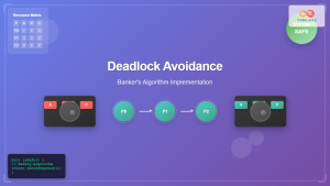
Deadlock Avoidance: Banker’s Algorithm Implementation and Examples
Introduction to Deadlock Avoidance Deadlock avoidance is a crucial concept in operating systems that prevents the system from entering an...
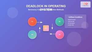
Deadlock in Operating System: Complete Guide to Necessary Conditions and Detection Methods
Deadlock is one of the most critical challenges in operating system design, where multiple processes become permanently blocked while waiting...

Resource Allocation Graph: Complete Guide to Deadlock Detection and Prevention
Resource Allocation Graphs (RAG) serve as powerful visual tools in operating systems for detecting and preventing deadlocks. This comprehensive guide...
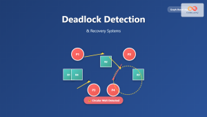
Deadlock Detection and Recovery: Graph-based Algorithms for Operating Systems
Introduction to Deadlock Detection and Recovery Deadlock is one of the most critical challenges in operating systems where multiple processes...

Deadlock Prevention: Complete Guide to Avoiding Circular Wait Conditions
Understanding Deadlock and Circular Wait Deadlock is one of the most critical issues in operating systems where two or more...

Wait-for Graph: Comprehensive Guide to Deadlock Detection in Distributed Systems
Introduction to Wait-for Graphs In distributed systems, deadlock detection remains one of the most critical challenges for maintaining system reliability...

Critical Section Problem: Complete Guide to Mutual Exclusion Solutions in Operating Systems
What is the Critical Section Problem? The critical section problem is a fundamental challenge in operating systems where multiple processes...
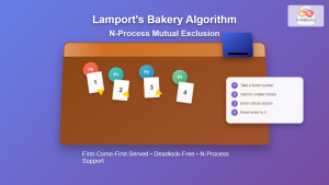
Lamport’s Bakery Algorithm: Complete Guide to N-Process Mutual Exclusion
Lamport's Bakery Algorithm stands as one of the most elegant solutions to the N-process mutual exclusion problem in concurrent programming....

Peterson’s Algorithm: Complete Guide to Two-Process Mutual Exclusion in Operating Systems
What is Peterson's Algorithm? Peterson's Algorithm is a classic solution for achieving mutual exclusion between two processes or threads in...

Memory Allocation Techniques: Contiguous vs Non-contiguous Management Strategies
Memory allocation is a fundamental aspect of operating system design that determines how programs and data are stored and accessed...

Lottery Scheduling: Fair CPU Allocation Through Proportional Sharing
Introduction to Lottery Scheduling Lottery scheduling is a probabilistic CPU scheduling algorithm that provides proportional share resource allocation by assigning...

Operating System Functions: Core Components and System Responsibilities
An operating system (OS) serves as the fundamental software layer that manages computer hardware resources and provides essential services to...