When designing and implementing algorithms, it is crucial to understand how well they perform in terms of efficiency. Performance is commonly analyzed in two dimensions: time complexity (how fast an algorithm runs) and space complexity (how much memory it uses). This detailed guide walks you through the fundamentals of algorithm complexity analysis, explains Big O notation with examples, and provides visuals to help you fully grasp the subject.
What is Algorithm Performance Analysis?
Algorithm performance analysis is the study of how the runtime or memory usage of an algorithm scales with input size. Rather than focusing on exact run times, which may vary depending on hardware and software environments, we use mathematical notations such as Big O, Big Ω, and Big Θ to describe behavior in terms of growth rates.
Key Aspects of Complexity
- Time Complexity: Measures the number of steps an algorithm takes to complete based on input size
n. - Space Complexity: Measures the amount of memory an algorithm requires during execution.
- Best Case, Average Case, Worst Case: Different perspectives on how an algorithm can perform depending on the inputs provided.
Big O Notation Explained
Big O notation is the most commonly used notation in complexity analysis. It provides an upper bound on runtime growth, helping us understand how an algorithm scales for large inputs.
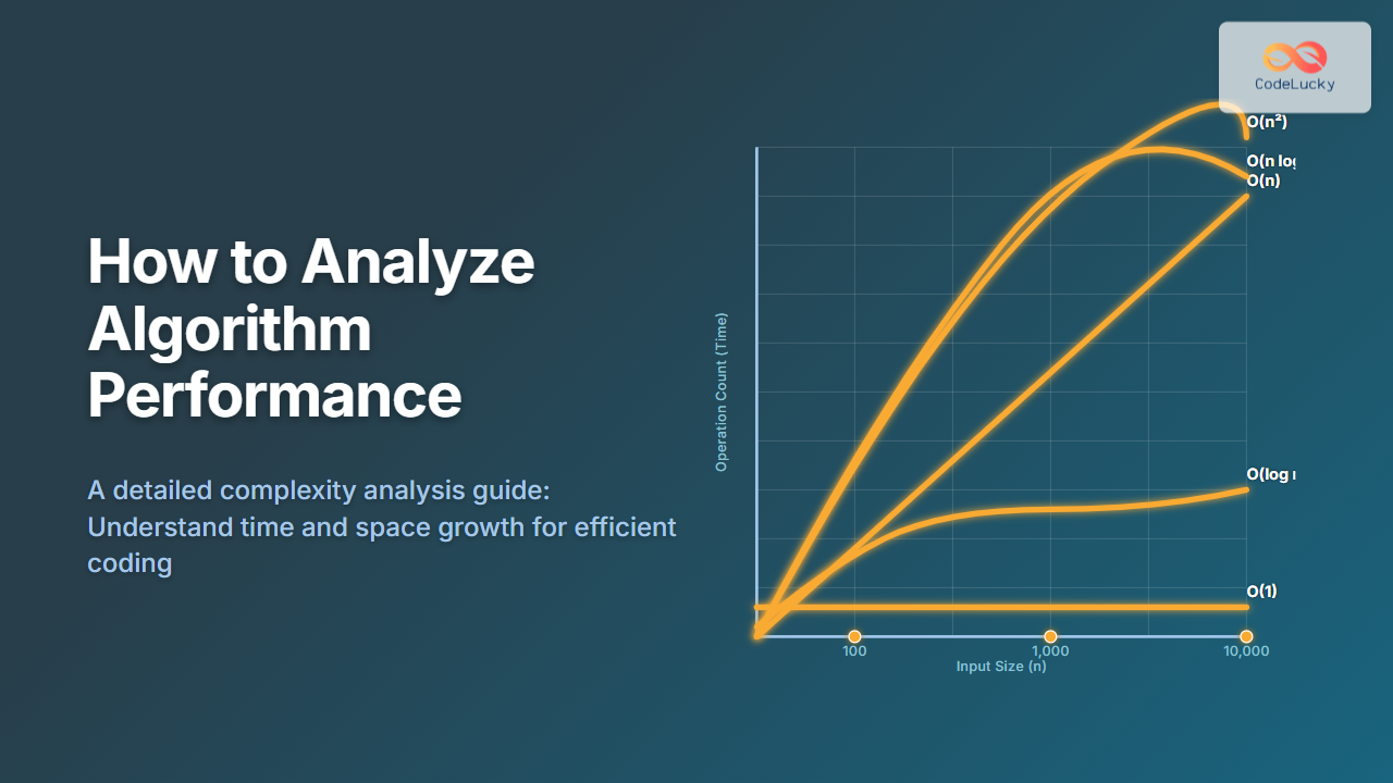
This diagram shows the relative increasing cost of different time complexities. As input size grows, exponential and factorial algorithms quickly become impractical.
Examples of Common Complexities
O(1) – Constant Time
A constant time operation does not depend on the input size.
void printFirstElement(int arr[]) {
    printf("%d\n", arr[0]);
}
No matter the size of the array, this function accesses the first element in constant time.
O(n) – Linear Time
Algorithms that must examine each element typically have linear time complexity.
def find_max(arr):
    max_val = arr[0]
    for val in arr:
        if val > max_val:
            max_val = val
    return max_val
The loop iterates through each element once, making complexity O(n).
O(log n) – Logarithmic Time
Algorithms that reduce the problem size by half each step (such as binary search) have logarithmic time complexity.
int binarySearch(int arr[], int target) {
    int left = 0, right = arr.length - 1;
    while (left <= right) {
        int mid = (left + right) / 2;
        if (arr[mid] == target) return mid;
        if (arr[mid] < target) left = mid + 1;
        else right = mid - 1;
    }
    return -1;
}
Binary search keeps halving the range of possibilities until it finds the element, making it highly efficient for sorted arrays.
O(n²) – Quadratic Time
Nested loops typically indicate quadratic time complexity.
for (int i = 0; i < n; i++) {
    for (int j = 0; j < n; j++) {
        cout << i * j << endl;
    }
}
Each iteration of the outer loop runs the entire inner loop, leading to O(n²) operations.
Visualizing Complexities
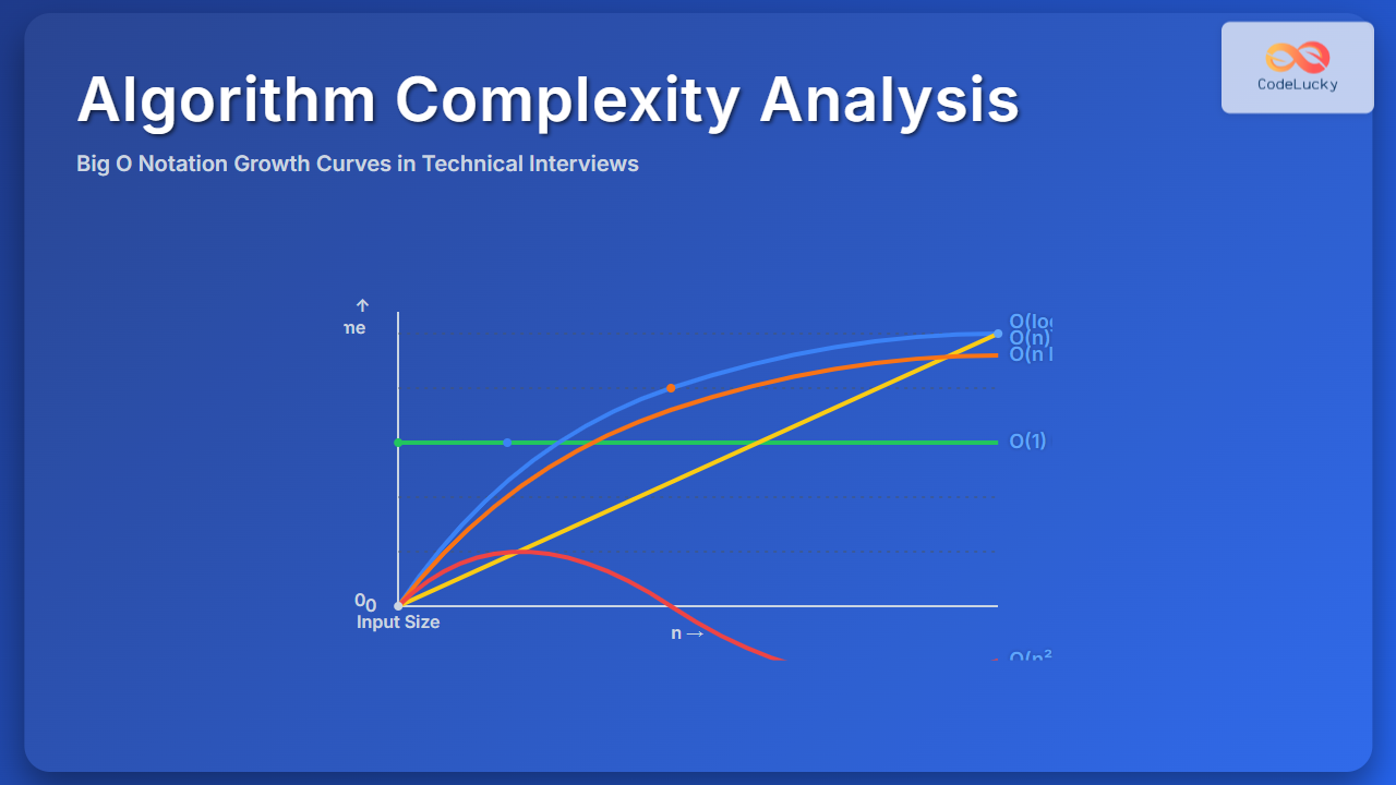
This visualization associates typical algorithms with their growth rates.
Space Complexity Examples
Sometimes reducing execution time requires more memory. Examples:
- O(1) Space: Binary search uses only a few variables, regardless of array size.
- O(n) Space: Storing all elements in recursion (such as Fibonacci with naive recursion).
Interactive Example: Time vs Input Size
Here is a small Python script you can try interactively to get a feel for growth rates:
import time

def linear_example(n):
    return sum(range(n))

def quadratic_example(n):
    total = 0
    for i in range(n):
        for j in range(n):
            total += i * j
    return total

for func in [linear_example, quadratic_example]:
    for n in [100, 1000, 5000]:
        start = time.time()
        func(n)
        end = time.time()
        print(f"{func.__name__} with n={n}: {(end - start):.5f} seconds")
Run this script and observe the difference in performance as n increases. You’ll notice that quadratic time grows much faster.
Why Algorithm Analysis Matters
- Predictability: Ensures your program won’t slow down dramatically with larger datasets.
- Optimization: Allows developers to choose better suited algorithms for large inputs.
- Scalability: Helps in building systems that can handle growth efficiently.
Conclusion
Mastering algorithm complexity analysis is essential for writing efficient programs. By studying Big O notation and understanding how input size affects runtime and memory usage, you prepare yourself for solving computing challenges effectively. Remember, the best algorithm is not always the one that “works,” but the one that scales efficiently as your input grows.
Use this guide as a reference to analyze, compare, and improve algorithms, and you will be well on your way to becoming a stronger problem solver and computer scientist.

