Algorithm Complexity Explained: Big O Notation Made Simple

Understanding algorithm complexity is fundamental for writing efficient software. In this article, Algorithm Complexity Explained: Big O Notation Made Simple, readers will learn how to evaluate algorithms by measuring their performance and resource consumption. This comprehensive guide covers crucial concepts behind Big O notation with clear examples, illustrative diagrams, and practical insights to empower developers in optimizing their code effectively.

Table of Contents

What Is Algorithm Complexity?

Algorithm complexity refers to the measurement of resources an algorithm consumes relative to input size, primarily focusing on time (how long it takes to run) and space (how much memory it uses). It helps predict and analyze an algorithm’s scalability and efficiency before actual implementation, crucial for performance-critical applications.

Introduction to Big O Notation

Big O notation is a mathematical representation that describes the upper bound of an algorithm’s running time or memory usage as input size approaches infinity. It simplifies comparisons by expressing complexity as a function of input size (n), focusing on dominant terms while ignoring constants and lower order terms.

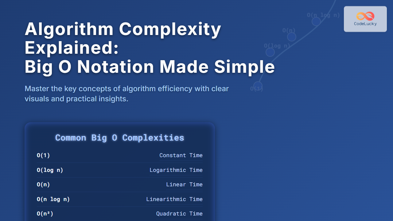
Common Big O Complexities

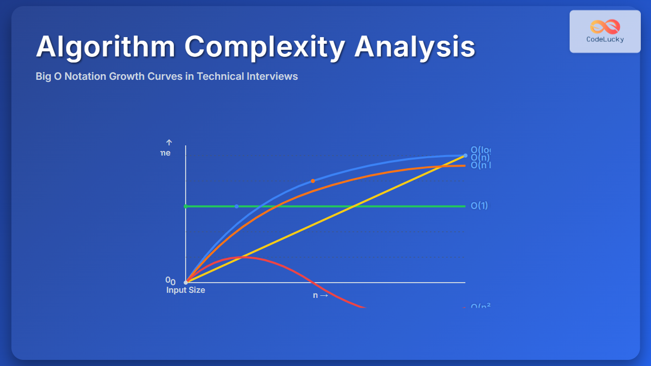
O(1) – Constant Time: Execution time stays the same regardless of input size.
O(log n) – Logarithmic Time: Execution time grows logarithmically, common in algorithms that halve the input (e.g., binary search).
O(n) – Linear Time: Execution time grows linearly with input size.
O(n log n) – Linearithmic Time: Algorithms like merge sort.
O(n²) – Quadratic Time: Time grows proportionally to the square of input size, common in nested loops.
O(2^n) – Exponential Time: Time doubles with each addition to input size, typical in algorithms exploring all combinations.

Example: Understanding Complexity with Code

Consider three common algorithm examples in Python and their time complexities.

1. Constant Time – O(1)

def get_first_element(arr):
    return arr[0]

This function returns the first element irrespective of the array size, so it runs in constant time O(1).

2. Linear Time – O(n)

def find_max(arr):
    max_val = arr[0]
    for num in arr:
        if num > max_val:
            max_val = num
    return max_val

Here, the function checks each element once, so time grows linearly with input size.

3. Quadratic Time – O(n²)

def print_pairs(arr):
    for i in range(len(arr)):
        for j in range(len(arr)):
            print(arr[i], arr[j])

This function has nested loops, resulting in n² iterations as input size grows.

Visualizing Algorithm Growth

Let’s visualize how time complexity grows with increasing input size (n):

Why Big O Matters

Understanding Big O enables developers to:

Predict algorithm performance at scale.
Choose the most efficient solution.
Optimize existing code by targeting expensive operations.
Communicate performance expectations clearly.

Tips for Analyzing Algorithm Complexity

Focus on dominant terms: Ignore constants and lower-order terms.
Differentiate worst, average, and best cases: Big O usually describes worst-case scenarios.
Consider both time and space complexity: Trade-offs might be necessary.
Analyze loops, recursion, and data access patterns: They often define complexity.

Summary

Big O notation is a fundamental concept for assessing and understanding algorithm complexity. It provides a standardized way to express how algorithms scale and perform, helping you write faster and more efficient code. By mastering Big O, developers can make informed decisions, optimize solutions, and enhance software quality effectively.