The A* Search Algorithm is one of the most widely used pathfinding and graph traversal techniques in computer science. Known for balancing efficiency and optimality, A* is popular in video games, robotics, maps, and artificial intelligence. Unlike Dijkstra’s algorithm which explores nodes purely based on cumulative cost or Greedy Best-First Search which relies solely on heuristic estimates, A* strikes a harmony by combining both approaches. This makes it ideal for real-world applications where we need fast and accurate results.
What is A* Search Algorithm?
A* (pronounced “A-star”) is a best-first search algorithm that finds the shortest path between nodes in a weighted graph. It works by considering two values for each node:
- g(n) → The cost of the path from the start node to current node n.
- h(n) → A heuristic estimate of the cost from n to the goal node.
- f(n) = g(n) + h(n) → The sum of the above two, used to prioritize which node to explore next.
The heuristic function h(n) guides the search towards the goal, while g(n) ensures that the solution is optimal.
How A* Works
A* uses two sets to manage search:
- Open Set: Nodes to be evaluated (priority queue sorted by f(n)).
- Closed Set: Nodes already evaluated.
Heuristic Functions in A*
The power of A* comes from its heuristic. Common heuristics include:
- Manhattan Distance: Used in grids with 4-directional moves:
abs(x1-x2)+abs(y1-y2). - Euclidean Distance: Used when diagonal movement is allowed:
sqrt((x1-x2)^2 + (y1-y2)^2). - Chebyshev Distance: For 8-direction movement:
max(abs(x1-x2), abs(y1-y2)).
Python Implementation of A* Search
Below is a simple Python implementation of A* on a grid:
import heapq
import math

def heuristic(a, b):
    # Using Manhattan Distance here
    return abs(a[0] - b[0]) + abs(a[1] - b[1])

def astar_search(start, goal, grid):
    rows, cols = len(grid), len(grid[0])
    open_set = []
    heapq.heappush(open_set, (0, start))

    came_from = {}
    g_score = {start: 0}

    while open_set:
        _, current = heapq.heappop(open_set)

        if current == goal:
            path = []
            while current in came_from:
                path.append(current)
                current = came_from[current]
            return path[::-1]  # reverse path

        neighbors = [(0,1),(0,-1),(1,0),(-1,0)]
        for dx, dy in neighbors:
            neighbor = (current[0] + dx, current[1] + dy)

            if 0 <= neighbor[0] < rows and 0 <= neighbor[1] < cols and grid[neighbor[0]][neighbor[1]] == 0:
                tentative_g = g_score[current] + 1

                if neighbor not in g_score or tentative_g < g_score[neighbor]:
                    came_from[neighbor] = current
                    g_score[neighbor] = tentative_g
                    f = tentative_g + heuristic(neighbor, goal)
                    heapq.heappush(open_set, (f, neighbor))

    return None
Example Execution
Consider a 5×5 grid where 0 represents free space and 1 represents walls:
grid = [
 [0,0,0,0,0],
 [1,1,0,1,0],
 [0,0,0,1,0],
 [0,1,1,1,0],
 [0,0,0,0,0]
]

path = astar_search((0,0), (4,4), grid)
print("Optimal Path:", path)
Output:
Optimal Path: [(0, 0), (0, 1), (0, 2), (1, 2), (2, 2), (2, 1), (2, 0), (3, 0), (4, 0), (4, 1), (4, 2), (4, 3), (4, 4)]
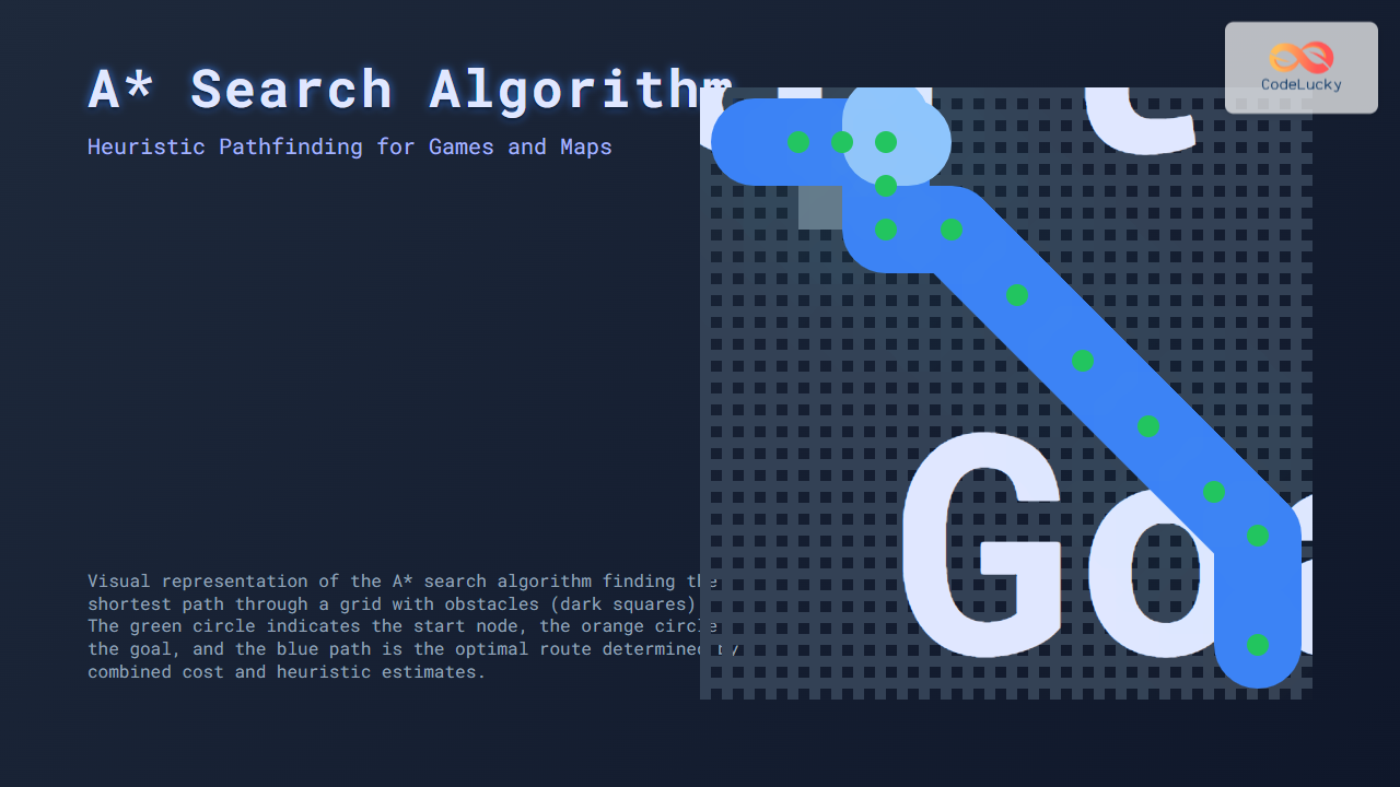
Visual Representation
Applications of A*
- Video Games: NPC navigation and obstacle avoidance.
- Maps and GPS: Route planning with road distances as weights.
- Robotics: Optimal movement planning in dynamic environments.
- AI: Puzzle solving and strategic simulations.
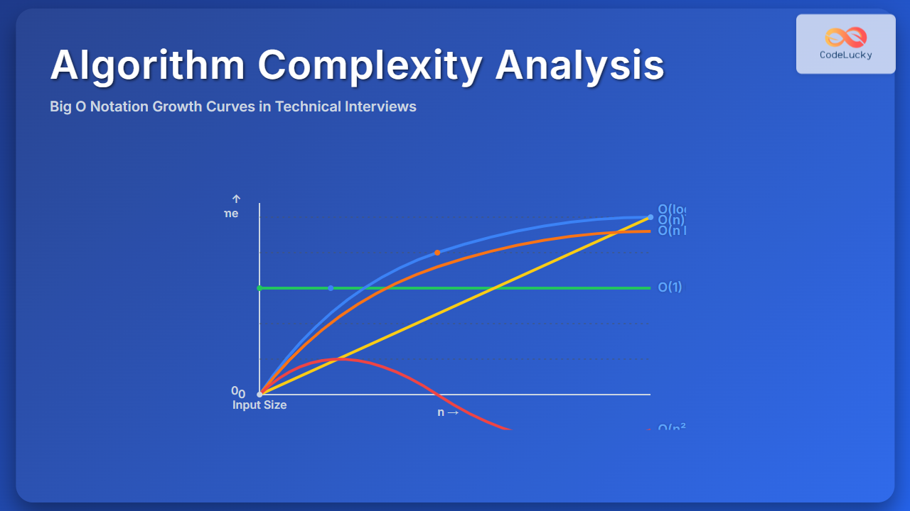
Complexity Analysis
- Time Complexity:
O(E)in worst case (similar to Dijkstra), but often much faster due to heuristic pruning. - Space Complexity:
O(V), storing g(n), h(n), and open/closed sets.
Conclusion
The A* Search Algorithm is an indispensable tool in pathfinding, merging the reliability of Dijkstra with the intelligence of heuristics. It is fast, optimal with admissible heuristics, and versatile enough to power everything from games to GPS navigation systems. With a strong understanding of heuristics and grid representation, programmers can implement highly efficient AI-driven movement systems using A*.


